Welcome
Dear Students,
Welcome to the programming course in theoretical chemistry. This class builds on the bachelor lecture "Programming Course for Chemists" and assumes that you are already familiar with the basic principles of Python and the numerical algorithms explained there.
According to current planning, the lecture will take place
- every Monday from 10:15 to 11:45
and the corresponding exercise
- every Thursday from 12:15 to 13:45.
Syllabus
A preliminary syllabus is shown below. This can and will be continously updated throughout the semester according to the progress.
| Week | Weekday | Date | Type | Topic |
|---|---|---|---|---|
| 1 | Mon. | Apr. 25 | Lecture | Fundamentals I |
| 1 | Thur. | Apr. 28 | Lecture | Fundamentals II |
| 2 | Mon | May 2 | Lecture | SymPy: Basics |
| 2 | Thur. | May 5 | Lecture | SymPy: Applications |
| 3 | Mon. | May 9 | Lecture | Fourier Transform I |
| 3 | Thur. | May 12 | Lecture | Fourier Transform II |
| 4 | Mon. | May 16 | Exercise | Exercise 0 |
| 4 | Thur. | May 19 | Lecture | Fourier Transform III |
| 5 | Mon. | May 23 | Exercise | Exercise 1 |
| 6 | Mon. | May 30 | Lecture | Fourier Transform IV |
| 6 | Thur. | Jun. 2 | Lecture | Eigenstates I |
| 7 | Thur. | Jun. 9 | Lecture | Eigenstates II |
| 8 | Mon. | Jun. 13 | Exercise | Exercise 2 |
| 9 | Mon. | Jun. 20 | Lecture | Eigenstates III |
| 9 | Thur. | Jun. 23 | Lecture | Eigenstates IV |
| 10 | Mon. | Jun. 27 | Lecture | Quantum Dynamics I |
| 11 | Mon. | Jul. 4 | Lecture | Quantum Dynamics II |
| 11 | Thur. | Jul. 7 | Lecture | Quantum Dynamics III |
| 12 | Mon. | Jul. 11 | Lecture | |
| 12 | Thur. | Jul. 14 | Lecture | |
| 13 | Mon. | Jul. 18 | Exercise | Exercise 3 |
| 13 | Thur. | Jul. 21 | ||
| 14 | Mon. | Jul. 25 | Lecture | |
| 14 | Thur. | Jul. 28 |
Technical notes
Python Distribution
We recommend to use an Anaconda or Miniconda Python environment. Your Python version for this class should be at least 3.5 or higher. The installation of Anaconda is also shown in the following video:
Integrated Development Environment (IDE) or Editor recommendations
-
- will be automatically available after you have installed Anaconda/Miniconda.
- if you are not yet familiar with Jupyter notebooks, you can find many tutorials in the web, e.g. Tutorial.
-
- is a full Python IDE with the focus on scientific development.
- will be automatically installed if you install the full Anaconda package.
-
- is a more lightweight text editor for coding purposes and one of the most used ones.
- Although it is officially not a real IDE, it has almost all features of an IDE.
-
- commercial (free for students) IDE with a lot of functionalities.
- is usually more suitable for very large and complex Python projects and can be too cumbersome for small projects like the ones used here in the lecture.
-
Vim/NeoVim
- command-line text editor which is usually pre installed on all unix-like computers.
- can be very unwieldy at the beginning, since Vim has a very large number of keyboard shortcuts and is not as beginner friendly as a typical IDE or Jupyter notebooks.
- is extremely configurable and can be adapted with a little effort to a very extensive and comfortable editor.
- still one of the most used editors.
During the lecture we will use different Python libraries. Therefore it is necessary that you install these libraries.
Dependencies
- NumPy
conda install matplotlib
- Matplotlib
conda install -c anaconda numpy
- SciPy
conda install -c anaconda scipy
- SymPy
conda install -c anaconda sympy
- pytest
conda install -c anaconda pytest
- ipytest
conda install -c conda-forge ipytest
- Hypothesis
conda install -c conda-forge hypothesis
Why Python?
Popularity
Python is one of the most widely used programming languages and is particularly beginner-friendly.
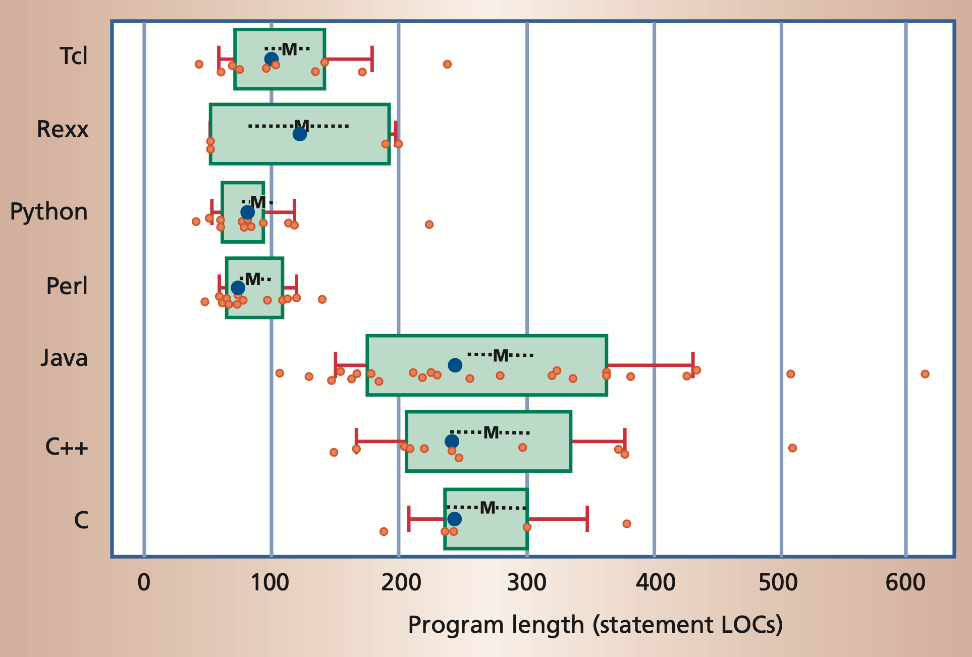
The following figure shows the popularity of some programming languages.
 Popularity of common programming languages. The popularities are taken
from the PYPL index
Popularity of common programming languages. The popularities are taken
from the PYPL index
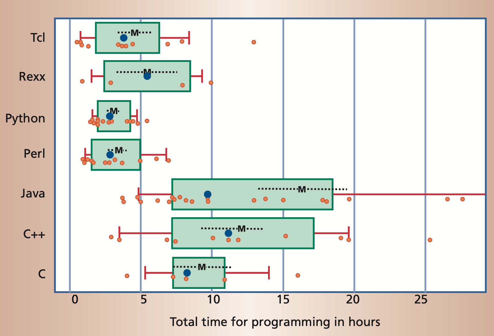
Requires often fewer lines of code and less work
Python often requires significantly fewer lines of code to implement
the same algorithms than compiled languages such as Java or C/C++.
 Program length, measured in number of noncomment source lines of code
(LOC).
Program length, measured in number of noncomment source lines of code
(LOC).
Moreover, it is often possible to accomplish the same task in significantly
less time in a scripting language than it takes using a compiled language.
But Python is slow!?
A common argument that is raised against using Python is that it is a comparatively slow language. There is some truth to this statement. Therefore, we want to understand one of the reasons why this is so and then explain why (in most cases) this is not a problem for us.
Python is an interpreted language.
Python itself is a C program that reads the source code of a text file, interprets it and executes it. This is in contrast to a compiled language like C, C++, Rust, etc. where the source code is compiled to machine code. The compiler has the ability to do lots of optimizations to the code which leads to a shorter runtime. This behavior can be shown by a simple example. Let's assume we have a naïve implementation to sum up all odd numbers up to 100 million:
s = 0
for i in range(100_000_000):
    if i % 2 == 1:
        s += i
This code takes about 8 seconds on my computer (M1 mac) to execute. Now we can implement the same algorithm in a compiled language to see the impact of the compiler. The following listing is written in a compiled language (Rust), but the details of this code and the programming language do not matter at this point:
#![allow(unused)]
fn main() {
let mut s: usize = 0;
for i in 0..100_000_000 {
    if i % 2 == 1 {
        s += i;
    }
}
}
This code has actually no runtime at all and evaluates instantaneously.
The compiler is smart enough to understand that everything can be
computed at compile time and just inserts the value for the variable
s. This now makes it clear that compiled languages can make use of
methods that interpreted languages lack simply by virtue of their
approach. However, we have seen before that compiled languages usually
require more lines of code and more work. In addition, there are usually
much more concepts to learn.
Python can be very performant
During this lecture we will often use Python libraries like NumPy or Scipy for mathematical algorithms and linear algebra in particular. These packages bring two big advantages. On the one hand they allow the use of complicated algorithms very easily and on the other hand these packages are written in compiled languages like C or Fortran. This way we can benefit from the performance advantages without having to learn another possibly more complicated language.
How to interact with this website
This section gives an introduction on how to interact with the lecture notes. These are organized into chapters. Each chapter is a separate page. Chapters are nested into a hierarchy of sub-chapters. Typically, each chapter will be organized into a series of headings to subdivide a chapter.
Navigation
There are several methods for navigating through the chapters of a book.
The sidebar on the left provides a list of all chapters. Clicking on any of the chapter titles will load that page.
The sidebar may not automatically appear if the window is too narrow, particularly on mobile displays. In that situation, the menu icon (three horizontal bars) at the top-left of the page can be pressed to open and close the sidebar.
The arrow buttons at the bottom of the page can be used to navigate to the previous or the next chapter.
The left and right arrow keys on the keyboard can be used to navigate to the previous or the next chapter.
Top menu bar
The menu bar at the top of the page provides some icons for interacting with the notes.
| Icon | Description |
|---|---|
| Opens and closes the chapter listing sidebar. | |
| Opens a picker to choose a different color theme. | |
| Opens a search bar for searching within the book. | |
| Instructs the web browser to print the set of notes. |
Tapping the menu bar will scroll the page to the top.
Search
The lecture notes have a built-in search system.
Pressing the search icon () in the menu bar or pressing the S key on the keyboard will open an input box for entering search terms.
Typing any terms will show matching chapters and sections in real time.
Clicking any of the results will jump to that section. The up and down arrow keys can be used to navigate the results, and enter will open the highlighted section.
After loading a search result, the matching search terms will be highlighted in the text.
Clicking a highlighted word or pressing the Esc key will remove the highlighting.
Code blocks
Code blocks contain a copy icon , that copies the code block into your local clipboard.
Here's an example:
print("Hello, World!")
We will often use the assert statement in code listings to show you
the value of a variable. Since the code blocks in this document are not
interactive (you can not simply execute them in your browser), it is
not possible to print the value of the variable to the screen.
Therefore, we ensure for you that all code blocks in these lecture notes
run without errors and in this way we can represent the value of a
variable through the use of assert.
The following code block for example shows that the variable a has
the value 2:
a = 2
assert a == 2
If the condition would evaluate to False, the assert statement would
raise an AssertionError.
Fundamentals
In the following sections we will explain the concept of bitwise operators, but first lay the necessary foundations. Our goal is to show what bitwise operators do and what they can be useful for. Afterwards, we also want to show the possibility and importance of unit tests. At the end of this chapter you should be able to answer the following questions:
- How are numbers represented in the computer?
- What is the difference in the representation between signed and unsigned numbers/integers?
- Which operations exist to compare the state of two bits?
- What are bitwise operators?
- What are unit tests? And why are they important?
Binary Numbers
When working with any kind of digital electronics it is important to understand that numbers are represented by two levels which can represent a one or a zero. The number system based on ones and zeroes is called the binary system (because there are only two possible digits). Before discussing the binary system, a review of the decimal (ten possible digits) system is helpful, because many of the concepts of the binary system will be easier to understand when introduced alongside their decimal counterpart.
Decimal System
You should all have some familiarity with the decimal system. For instance, to represent the positive integer one hundred and twenty-five as a decimal number, we can write (with the postive sign implied):
$$ 125_{10} = 1 \cdot 100 + 2 \cdot 10 + 5 \cdot 1 = 1 \cdot 10^2 + 2 \cdot 10^1 + 5 \cdot 10^0 $$
The subscript 10 denotes the number as a base 10 (decimal) number.
There are some important observations:
- To multiply a number by 10 you can simply shift it to the left by one digit, and fill in the rightmost digit with a 0 (moving the decimal place one to the right).
- To divide a number by 10, simply shift the number to the right by one digit (moving the decimal place one to the left).
- To see how many digits a number needs, you can simply take the logarithm (base 10) of the absolute value of the number, and add 1 to it. The integral part of the result will be the number of digits. For instance, \(\log_{10}(33) + 1 = 2.5.\)
Binary System (of positive integers)
Binary representations of positive integers can be understood in the same way as their decimal counterparts. For example
$$ 86_{10}=1 \cdot 64+0 \cdot 32+1 \cdot 16+0 \cdot 8+1 \cdot 4+1 \cdot 2+0 \cdot 1 $$
This can also be written as:
$$ 86_{10}=1 \cdot 2^{6} +0 \cdot 2^{5}+1 \cdot 2^{4}+0 \cdot 2^{3}+1 \cdot 2^{2}+1 \cdot 2^{1}+0 \cdot 2^{0} $$ or
$$ 86_{10}=1010110_{2} $$
The subscript 2 denotes a binary number. Each digit in a binary number is called a bit. The number 1010110 is represented by 7 bits. Any number can be broken down this way, by finding all of the powers of 2 that add up to the number in question (in this case \(2^6\), 2\(^4\), 2\(^2\) and 2\(^1\)). You can see this is exactly analogous to the decimal deconstruction of the number 125 that was done earlier. Likewise we can make a similar set of observations:
- To multiply a number by 2 you can simply shift it to the left by one digit, and fill in the rightmost digit with a 0.
- To divide a number by 2, simply shift the number to the right by one digit.
- To see how many digits a number needs, you can simply take the logarithm (base 2) of the number, and add 1 to it. The integral part of the result is the number of digits. For instance, \(\log_{2}(86) + 1 = 7.426.\) The integral part of that is 7, so 7 digits are needed. With \(n\) digits, \(2^n\) unique numbers (from 0 to \(2^n - 1\)) can be represented. If \(n=8\), 256 (\(=2^8\)) numbers can be represented (0-255).
This counter shows how to count in binary from zero through thirty-one.
Binary System of Signed Integers
We will not be using a minus sign (\(-\)) to represent negative numbers. We would like to represent our binary numbers with only two symbols, 0 and 1. There are a few ways to represent negative binary numbers. We will discuss each of these in the following subsections.
Note: Unlike other programming languages, where different types of integers exist (signed, unsigned, different number of bits), in Python there is only one integer type (
int). This is a signed integer type with arbitrary precision. This means, the integer has not a fixed number of bits to represent the number, but will dynamically use as many bits as needed to represent the number. Therefore, integer overflows cannot occur in Python. This doesn't hold forfloats, which have fixed size of 64 bit and can overflow.
Sign and Magnitude
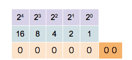
The most significant bit (MSB) determines if the number is positive (MSB is 0) or negative (MSB is 1). All following bits are the so called magnitude bits. This means that a 8 bit signed integer can represent all numbers from -127 to 127 (\(-2^6\) to \(2^6\)). Except for the MSB, all positive and negative numbers share the same representation.

Visualization of the Sign and Magnitude representation of the decimal number +13.
In the case of a negative number, the only difference is that the first bit (the MSB) is inverted, as shown in the following Scheme.

Visualization of the Sign and Magnitude representation of the decimal number -31
Although this representation seems very intimate and simple, there are multiple consequences and problems that it makes:
- There are two ways to represent zero,
0000 0000and1000 0000. - Addition and subtraction require different behaviors depending on the sign bit.
- Comparisons (e.g. greater, less, ...) also require inspection of the sign bit.
This approach is directly comparable to the common way of showing a sign (placing a "+" or "−" next to the number's magnitude). This kind of representation was only used in early binary computers and was replaced by representations that we will discuss in the following.
Ones' Complement
To overcome the limitations of the Sign and Magnitude representation, another representation was developed with the following idea in mind: One wants to flip the sign of an integer by inverting all bits.
This inversion is also known as taking the complement of the bits. The implication of this idea is, that the first bit, the MSB, also represents just the sign as in the Sign and Magnitude case. However, the decimal value of all other bits are now dependent of the MSB bit state. It might be easier to understand this behaviour by a simple example that outlines the motivation again.
We want that our binary representation behaves like:

The advantage of this representation is that for adding two numbers, one can do a conventional binary addition, but it is then necessary to do an end-around carry: that is, add any resulting carry back into the resulting sum. To see why this is necessary, consider the following example showing the case of the following addition $$ −1_{10} + 2_{10} $$
or
$$ 1111 1110_2 + 0000 0010_2 $$

In the previous example, the first binary addition gives 00000000, which
is incorrect. The correct result (00000001) only appears when the carry
is added back in.
A remark on terminology: The system is referred to as ones' complement because the negation of a positive value x (represented as the bitwise NOT of x, we will discuss the bitwise NOT in the following sections) can also be formed by subtracting x from the ones' complement representation of zero that is a long sequence of ones (−0).
Two's Complement
In the two's complement representation, a negative number is represented by the bit pattern corresponding to the bitwise NOT (i.e. the "complement") of the positive number plus one, i.e. to the ones' complement plus one. It circumvents the problems of multiple representations of 0 and the need for the end-around carry of the ones' complement representation.
This can also be thought of as the most significant bit representing the inverse of its value in an unsigned integer; in an 8-bit unsigned byte, the most significant bit represents the number 128, where in two's complement that bit would represent −128.

In two's-complement, there is only one zero, represented as 00000000. Negating a number (whether negative or positive) is done by inverting all the bits and then adding one to that result.
Addition of a pair of two's-complement integers is the same as addition of a pair of unsigned numbers. The same is true for subtraction and even for N lowest significant bits of a product (value of multiplication). For instance, a two's-complement addition of 127 and −128 gives the same binary bit pattern as an unsigned addition of 127 and 128, as can be seen from the 8-bit two's complement table.

Two's complement is the representation that Python uses for it's type
int.
Logic Gates
Truth tables show the result of combining inputs using a given operator.
NOT Gate
The NOT gate, a logical inverter, has only one input. It reverses the logic state. If the input is 0, then the output is 1. If the input is 1, then the output is 0.
| INPUT | OUTPUT |
|---|---|
| 0 | 1 |
| 1 | 0 |
AND Gate
The AND gate acts in the same way as the logical "and" operator. The following truth table shows logic combinations for an AND gate. The output is 1 only when both inputs are 1, otherwise, the output is 0.
| A | B | Output |
|---|---|---|
| 0 | 0 | 0 |
| 0 | 1 | 0 |
| 1 | 0 | 0 |
| 1 | 1 | 1 |
OR Gate
The OR gate behaves after the fashion of the logical inclusive "or". The output is 1 if either or both of the inputs are 1. Only if both inputs are 0, then the output is 0.
| A | B | Output |
|---|---|---|
| 0 | 0 | 0 |
| 0 | 1 | 1 |
| 1 | 0 | 1 |
| 1 | 1 | 1 |
NAND Gate
The NAND gate operates as an AND gate followed by a NOT gate. It acts in the manner of the logical operation "and" followed by negation. The output is 0 if both inputs are 1. Otherwise, the output is 1.
| A | B | Output |
|---|---|---|
| 0 | 0 | 1 |
| 0 | 1 | 1 |
| 1 | 0 | 1 |
| 1 | 1 | 0 |
NOR Gate
The NOR gate is a combination of OR gate followed by a NOT gate. Its output is 1 if both inputs are 0. Otherwise, the output is 0.
| A | B | Output |
|---|---|---|
| 0 | 0 | 1 |
| 0 | 1 | 0 |
| 1 | 0 | 0 |
| 1 | 1 | 0 |
XOR Gate
The XOR (exclusive-OR) gate acts in the same way as the logical "either/or." The output is 1 if either, but not both, of the inputs are 1. The output is 0 if both inputs are 0 or if both inputs are 1. Another way of looking at this circuit is to observe that the output is 1 if the inputs are different, but 0 if the inputs are the same.
| A | B | Output |
|---|---|---|
| 0 | 0 | 0 |
| 0 | 1 | 1 |
| 1 | 0 | 1 |
| 1 | 1 | 0 |
XNOR Gate
The XNOR (exclusive-NOR) gate is a combination of XOR gate followed by a NOT gate. Its output is 1 if the inputs are the same, and 0 if the inputs are different.
| A | B | Output |
|---|---|---|
| 0 | 0 | 1 |
| 0 | 1 | 0 |
| 1 | 0 | 0 |
| 1 | 1 | 1 |
Bitwise Operators
Bitwise operators are used to manipulate the states of bits directly. In Python (>3.5) there are 6 bitwise operators defined:
| Operator | Name | Example | Output (x=7, y=2) |
|---|---|---|---|
| << | left bitshift | x << y | 28 |
| >> | right bitshift | x >> y | 1 |
| & | bitwise and | x & y | 2 |
| | | bitwise or | x | y |
| ~ | bitwise not | ~x | -8 |
| ^ | bitwise xor | x ^ y | 5 |
Left Bitshift
Returns x with the bits shifted to the left by y places (and new bits on the right-hand-side are zeros). This is the same as multiplying \(x\) by \(2^y\).
The easiest way to visualize this operation is to consider a number that consists of only a single 1 in binary representation. If we now simply shift a 1 to the left three times in succession, we get the following:
assert (1 << 1) == 2  # ..0001 => ..0010
assert (2 << 1) == 4  # ..0010 => ..0100
assert (4 << 1) == 8  # ..0100 => ..1000
But we can also do this operation with just one call:
assert (1 << 3) == 8 # ..0001 => ..1000
Of course, we can also apply this operation to any other number:
assert (3 << 2) == 12 # ..0011 => ..1100
Right Bitshift
Returns x with the bits shifted to the right by y places. This is the same as dividing \(x\) by \(2^y\).
assert (8 >> 1) == 4 # ..1000 => ..0100
assert (4 >> 1) == 2 # ..0100 => ..0010
assert (2 >> 1) == 1 # ..0010 => ..0001
As we did with the bit shift to the left side, we can also shift a bit multiple times to the right:
assert (8 >> 3) == 1 # ..1000 => ..0001
Or apply the operator to any other number that is not a multiple of 2.
assert (11 >> 2) == 2 # ..1011 => ..0010
Bitwise AND
Does a "bitwise and". Each bit of the output is 1 if the corresponding bit of \(x\) AND \(y\) is 1, otherwise it is 0.
assert (1 & 2) == 0  # ..0001 & ..0010 => ..0000
assert (7 & 5) == 5  # ..0111 & ..0101 => ..0101
assert (12 & 3) == 0 # ..1100 & ..0011 => ..0000
Bitwise OR
Does a "bitwise or". Each bit of the output is 0 if the corresponding bit of \(x\) OR \(y\) is 0, otherwise it's 1.
assert (1 | 2) == 3   # ..0001 & ..0010 => ..0011
assert (7 | 5) == 7   # ..0111 & ..0101 => ..0111
assert (12 | 3) == 15 # ..1100 & ..0011 => ..1111
Bitwise NOT
Returns the complement of \(x\) - the number you get by switching each 1 for a 0 and each 0 for a 1. This is the same as \(-x - 1\).
assert ~0 == -1
assert ~1 == -2
assert ~2 == -3
assert ~3 == -4
Bitwise XOR
Does a "bitwise exclusive or". Each bit of the output is the same as the corresponding bit in \(x\) if that bit in \(y\) is 0, and it is the complement of the bit in x if that bit in y is 1.
assert (1 ^ 2) == 3   # ..0001 & ..0010 => ..0011
assert (7 ^ 5) == 2   # ..0111 & ..0101 => ..0010
assert (12 ^ 3) == 15 # ..1100 & ..0011 => ..1111
Arithmetic Operators
Arithmetic operators are used to perform mathematical operations like addition, subtraction, multiplication and division. In Python (>3.5) there are 7 arithmetic operators defined:
| Operator | Name | Example | Output (x=7, y=2) |
|---|---|---|---|
| + | Addition | x + y | 9 |
| - | Subtraction | x - y | 5 |
| * | Multiplication | x * y | 14 |
| / | Division | x / y | 3.5 |
| // | Floor division | x // y | 3 |
| % | Modulus | x % y | 1 |
| ** | Exponentiation | x ** y | 49 |
Addition
The + (addition) operator yields the sum of its arguments.
The arguments must either both be numbers or both be sequences of the same type. Only in the former case, the numbers are converted to a common type and a arithmetic addition is performed. In the latter case, the sequences are concatenated, e.g.
a = [1, 2, 3]
b = [4, 5, 6]
assert (a + b) == [1, 2, 3, 4, 5, 6]
Subtraction
The - (subtraction) operator yields the difference of its arguments.
The numeric arguments are first converted to a common type.
Note: In contrast to the addition, the subtraction operator cannot be applied to sequences.
Multiplication
The * (multiplication) operator yields the product of its arguments.
The arguments must either both be numbers, or one argument must be an integer and the other must be a sequence.
In the former case, the numbers are converted to a common type and then multiplied together.
In the latter case, sequence repetition is performed; e.g.
a = [1, 2]
assert (3 * a) == [1, 2, 1, 2, 1, 2]
Note: a negative repetition factor yields an empty sequence; e.g.
a = 3 * [1, 2]
assert (-2 * a) == []
Division & Floor division
The / (division) and // (floor division) operators yield the quotient of their arguments.
The numeric arguments are first converted to a common type.
Note: Division of integers yields a float, while floor division of integers results in an integer;
the result is that of mathematical division with the floor function applied to the result.
Division by zero raises a ZeroDivisionError exception.
Modulus
The % (modulo) operator yields the remainder from the division of the first argument by the second.
The numeric arguments are first converted to a common type.
A zero right argument raises the ZeroDivisionError exception.
The arguments may even be floating point numbers, e.g.,
import math
assert math.isclose(3.14 % 0.7, 0.34)
# since
assert math.isclose(3.14, 4*0.7 + 0.34)
The modulo operator always yields a result with the same sign as its second operand (or zero); the absolute value of the result is strictly smaller than the absolute value of the second operand.
Note: As you may have noticed in the listing above, we did not use the comparison operator
==to test the equality of two floats. Instead we imported themathpackage and used the built-in isclose function. If you want to read more detailed information about float representation errors the following blog post can be recommended.
Exponentiation
The ** (power) operator has the same semantics as the built-in pow() function, when called with two arguments:
it yields its left argument raised to the power of its right argument. The numeric arguments are first converted to a common type.
The result type is that of the arguments after coercion;
if the result is not expressible in that type (as in raising an integer to a negative power)
the result is expressed as a float (or complex).
In an unparenthesized sequence of power and unary operators, the operators are evaluated from right to left
(this does not constrain the evaluation order for the operands), e.g.
assert 2**2**3 == 2**(2**3) == 2**8 == 256
Implementation: Arithmetic Operators
All arithmetic operators can be implemented using bitwise operators. While addition and subtraction are implemented through hardware, the other operators are often realized via software. In this section, we shall implement multiplication and division for positive integers using addition, subtraction and bitwise operators.
Implementation: Multiplication
The multiplication of integers may be thought as repeated addition; that is, the multiplication of two numbers is equivalent to the following sum: $$ A \cdot B = \sum_{i=1}^{A} B $$ Following this idea, we can implement a naïve multiplication:
def naive_mul(a, b):
    r = 0
    for i in range(0, a):
        r += b
    return r
Although we could be smart and reduce the number of loops by choosing the smaller one to be the multiplier, the number of additions always grows linearly with the size of the multiplier. Ignoring the effect of multiplicand, this behavior is called linear-scaling, which is often denoted as \(\mathcal{O}(n)\).
Can we do better?
We have learned that multiplication by powers of 2 can be easily realized by
the left shift operator <<. Since every integer can be written as sum of
powers of 2, we may try to compute the necessary products of the multiplicand
with powers of 2 and sum them up. We shall do an example: 11 * 3.
assert (2**3 + 2**1 + 2**0) * 3 == 11 * 3
assert (2**3 * 3 + 2**1 * 3 + 2**0 *3) == 11 * 3
assert (3 << 3) + (3 << 1) + 3 == 11 * 3
To implement this idea, we can start from the multiplicand (b) and check the
least-significant-bit (LSB) of the multiplier (a). If the LSB is 1, this power of
2 is present in a and b will be added to the result. If the LSB is 0, this power is
not present in a and nothing will be done. In order to check the second LSB of a
and perhaps add 2 * b, we can just right shift a. In this way the second LSB
will become the new LSB and b needs to be multiplied by 2 (left shift).
This algorithm is illustrated for the example above as:
| Iteration | a | b | r | Action |
|---|---|---|---|---|
| 0 | 1011 | 000011 | 000000 | r += b, b <<= 1, a >>= 1 |
| 1 | 0101 | 000110 | 000011 | r += b, b <<= 1, a >>= 1 |
| 2 | 0010 | 001100 | 001001 | b <<= 1, a >>= 1 |
| 3 | 0001 | 011000 | 001001 | r += b, b <<= 1, a >>= 1 |
| 4 | 0000 | 110000 | 100001 | Only zeros in a. Stop. |
An example implementation is given in the following listing:
def mul(a, b):
    r = 0
    for _ in range(0, a.bit_length()):
        if a & 1 != 0:
            r += b
        b <<= 1
        a >>= 1
    return r
This new algorithm should scale with the length of the binary representation of the multiplier, which grows logarithmically with its size. This is denoted as \(\mathcal{O}(\log(n))\).
To show the difference between these two algorithms, we can write a function
to time their executions. The following example uses the function
perf_counter from time module:
    from random import randrange
    from time import perf_counter

    def time_multiplication(func, n, cycles=1):
        total_time = 0.0
        for i in range(0, cycles):
            a = randrange(0, n)
            b = randrange(0, n)

            t_start = perf_counter()
            func(a, b)
            t_stop = perf_counter()

            total_time += (t_stop - t_start)

        return total_time / float(cycles)
The execution time per execution for different sizes are listed below:
n | naive_mul / μs | mul / μs |
|---|---|---|
10 | 0.48 | 0.80 |
100 | 2.83 | 1.56 |
1 000 | 28.83 | 1.88 |
10 000 | 224.33 | 2.02 |
100 000 | 2299.51 | 2.51 |
Although the naïve algorithm is faster for \(a,b \leq 10\), its time
consumption grows rapidly when a and b become larger. For even larger
numbers, it will quickly become unusable. The second algorithm, however,
scales resonably well to be applied for larger numbers.
Implementation: Division
Just like for multiplication, the integer (floor) division may be treated as repeated subtractions. The quotient \( \lfloor A/B \rfloor \) tells us how often \(B\) can be subtracted from \(A\) before it becomes negative.
The naïve floor division can thus be implemented as:
def naive_div(a, b):
    r = -1
    while a >= 0:
        a -= b
        r += 1
    return r
Just like naïve multiplication, this division algorithm scales linearly with the size of dividend, if the effect of divisor is ignored.
Can we do better?
In school, we have learned to do long divisions. This can also be done
using binary numbers. We at first left-align the divisor b with the
dividend a and compare the sizes of the overlapping part. If the divisor is
smaller, it goes once into the dividend. Therefore, the quotient at that bit
becomes 1 and the dividend is subtracted from the part of divisor. Otherwise, this
quotient bit will be 0 and no subtraction takes place. Afterwards,
the dividend is right-shifted and the whole process repeated.
This algorithm is illustrated in the following table for the example 11 // 2:
| Iteration | a | b | r | Action |
|---|---|---|---|---|
| preparation | 1011 | 0010 | 0000 | b <<= 2 |
| 0 | 1011 | 1000 | 0000 | a -= b, r.2 = 1, b >>= 1 |
| 1 | 0011 | 0100 | 0100 | b >>= 1 |
| 2 | 0011 | 0010 | 0100 | a -= b, r.0 = 1, b >>= 1 |
| 3 | 0001 | 0001 | 0101 | Value of b smaller than initial. Stop. |
An example implementation is given in the following listing:
def div(a, b):
    n = a.bit_length()
    tmp = b << n
    r = 0
    for _ in range(0, n + 1):
        r <<= 1
        if tmp <= a:
            a -= tmp
            r += 1
        tmp >>= 1
    return r
In this implementation, rather than setting the result bitwise like described
in the table above, it is initialized to 0 and appended with 0 or 1.
Also, the divisor is shifted by the bit-length of a instead of the difference
between a and b. This may increase the number of loops, but prevents
negative shifts, when bit-length of a is smaller than that of b.
This algorithm is linear in the bit-length of the dividend and thus a \(\mathcal{\log(n)}\) algorithm. Again, we want to quantify the performance of both algorithms by timing them.
Since the size of the divisor does not have a simple relation with the
execution time, we shall fix its size. Here we choose nb = 10. An example
function for timing is shown in the following listing:
    from random import randrange
    from time import perf_counter

    def time_division(func, na, nb, cycles=1):
        total_time = 0.0
        for i in range(0, cycles):
            a = randrange(0, na)
            b = randrange(1, nb)

            t_start = perf_counter()
            func(a, b)
            t_stop = perf_counter()

            total_time += (t_stop - t_start)

        return total_time / float(cycles)
Since we cannot divide by zero, the second argument, the divisor in this case, is chosen between 1 and n instead of 0 and n.
The execution time per execution for different sizes are listed below:
na | naive_div / μs | div / μs |
|---|---|---|
10 | 0.38 | 1.06 |
100 | 1.54 | 1.67 |
1 000 | 13.79 | 1.83 |
10 000 | 117.20 | 1.89 |
100 000 | 1085.89 | 2.24 |
Again, although the naïve method is faster for smaller numbers, its scaling prevents it from being used for larger numbers.
Edge Cases
Division by zero
Since division by zero is not defined, we should handle the case, where the
user calls the division function with 0 as divisor. Both implemented division algorithms
would be stuck in the while loop if 0 is
passed as the second argument and thus block further commands from being
executed. We obviously do not want this to happen.
In general, there are two ways to deal with "forbidden" values. The first
one is to raise an error, just like the build-in division operators, which
raises a ZeroDivisionError and halts the program. This is realized by adding
an if-condition at the beginning of the algorithm:
def div_err(a, b):
    if b == 0:
        raise ZeroDivisionError
    ...
Sometimes, however, we want the program to continue even after encountering
forbidden values. In this case, we can make the algorithm return something,
which is recognizable as invalid. This way, the user can be informed about
forbidden values through the outputs. One possible choice of such invalid
object is the None object and can be used like
def div_none(a, b):
    if b == 0:
        return None
    ...
Negative input
While implementing multiplication and division algorithms, the problems were only analyzed using non-negative integers. Inputs of negative integers may therefore lead to undefined behaviors. Again, we can raise an exception when this happens or utilise an invalid object. The following listings show both cases on the multiplication algorithm:
def mul_err(a, b):
    if a < 0 or b < 0:
        raise ValueError
    ...
def mul_none(a, b):
    if a < 0 or b < 0:
        return None
    ...
These lines can be directly added to division algorithms to deal with negative inputs.
Floating-point input
Just like in the case of negative input values, floating-point numbers as
inputs may also lead to undefined behaviors. Although the same input guards
can be applied to deal with floating-point numbers, a more sensible way would
be to convert the input values to integer using int function before
executing the algorithms.
Unit Tests
Everybody makes mistakes. Although the computer which executes programs does exactly what it is told to, we can make mistakes which may cause unexpected behavior. Therefore, proper testing is mandatory for any serious application. But I can just try some semi-randomly picked inputs after writing a function and see if I get the expected output, so ...
Why bother with writing tests?
First of all, if you share your program with other people, you have to persuade them that your program works properly. It is far more convincing if you have written tests, which they can run for themselves and see that nothing is out of order, than just tell them that you have tested some hand-picked examples.
Furthermore, functions are often rewritten multiple times to improve their performance. Since you want to ensure that the function still works properly after even the slightest modification, you will have to run the manual tests over and over again. The problem only gets worse for larger projects. Nested conditions, interdependent modules, multiple inheritance, just to name a few, will make manual testing a horrible choice; even the tiniest change could make you re-test every routine you have written.
So, to make your (and other's) life easier, just write tests.
What are unit tests?
Unit tests are typically automated tests to ensure that a part of a program (known as a "unit") behaves as intended. A unit could be an entire module, but it is more commonly an individual function or an interface, such as a class.
Since unit tests focus on a specific part of the program, it is very good at isolating individual parts and find errors in them. This can accelerate the debugging process, since only the code of units corresponding to failed tests have to be inspected. Exactly due to this isolating action however, unit tests cannot be used to evaluate every execution path in any but the most trivial programs and will not catch every error. Nevertheless, unit tests are really powerful and can greatly reduce the number of errors.
Writing example based tests
Note: Since we want to discover errors using unit tests, let us assume that we did not discuss anything about the edge cases for multiplication and division routines we have written.
Although Python has the built-in module unittest, another framework for
unit tests, pytest, exists,
which is easier to use and offers more functionalities. Therefore, we will
stick to pytest in this class. The thoughts presented however,
can be used with any testing framework.
When using jupyter-notebook, the module
ipytestcould be very handy. This can be installed withconda install -c conda-forge ipytest
Using conda, we can install pytest by executing
conda install -c anaconda pytest
in the console.
Suppose we have written mul function in the file multiplication.py
and div function in the file division.py, we can create the file
test_mul_div_expl.py in the same directory and import both functions as:
from multiplication import mul
from division import div
Unit test with examples
We choose one example for each function and write
def test_mul_example():
    assert mul(3, 8) == 24

def test_div_example():
    assert div(17, 3) == 5
where we call each function on the selected example and compare the output with the expected outcome.
After saving and exiting the document, we can execute
pytest
in the console. pytest will then find every .py files in the directory
which begins with test execute every function inside, which begins with
test. If we only want to execute test functions from one specific file,
say, test_mul_div_expl.py. we should call
pytest test_mul_div_expl.py
If any assert statement throws an exception, pytest will informs
us about it. In this case, we should see
================================ 2 passed in 0.10s ================================although the time may differ. It is good to see that the test passed. but
just because something works on one example, does not mean it always works.
One way to be more confident is to go through more examples. Instead of
writing the same function for all examples, we can use the function decorator
@parametrize provided by pytest.
Unit test with parametrized examples
We can use the function decorator by importing pytest and write
import pytest

@pytest.mark.parametrize(
    'a, b, expected',
    [(3, 8, 24), (7, 4, 28), (14, 11, 154), (8, 53, 424)],
)
def test_mul_param_example(a, b, expected):
    assert mul(a, b) == expected

@pytest.mark.parametrize(
    'a, b, expected',
    [(17, 3, 5), (21, 7, 3), (31, 2, 15), (6, 12, 0)],
)
def test_div_param_example(a, b, expected):
    assert div(a, b) == expected
The decorator @parametrize feeds the test function with values and makes
testing with multiple examples easy. It will becomes tedious however, if
we want to try even more examples.
Unit test with random examples
By going through a large amount of randomly generated examples, we may
uncover rarely occuring errors. This method is not always available, since
the expected output must somehow be available. In this case however, we can
just use python's built-in * and // operator to verify our own
function.
The following listing shows tests for 50 examples:
from random import randrange

N = 50

def test_mul_random_example():
    for _ in range(0, N):
        a = randrange(1_000)
        b = randrange(1_000)
        assert mul(a, b) == a * b

def test_div_random_example():
    for _ in range(0, N):
        a = randrange(1_000)
        b = randrange(1_000)
        assert div(a, b) == a // b
Running pytest should probably give us 2 passes. To be more confident, we
can increase the number of loops to, say, 700. Now, calling pytest several
times, we might get something like
========================================= short test summary info ==========================================
FAILED test_mul_div.py::test_div_random_example -  ZeroDivisionError: integer division or modulo by zero
======================================= 1 failed, 1 passed in 0.20s =======================================
This tells us that the ZeroDivisonError exception occured while running
test_div_param_example function. Some more information can be seen above
the summary, and it should look like
def test_div_random_example():
        for _ in range(0, N):
            a = randrange(1_000)
            b = randrange(1_000)
>           assert div(a, b) == a // b
E          ZeroDivisionError: integer division or modulo by zero
The arrow in the second last line shows the code where the exception occured.
In this case, we have provided the floor division operator // with a zero
on the right side. We thus know that we should modify our own implementation
to handle this case.
We have found the error without knowing the detailed implementation of the functions. This is desired since human tends to overlook things when analyzing code and some special cases might not be covered by testing with just a few examples. Although with 700 loops, the test passes about 50 % of the time, if we increase the number of loops to several thousands or even higher, the test is almost guaranteed to fail and inform us about deficies in our functions.
The existence of a reference method is not only possible in our toy example,
but also occurs in realistic cases. A common case is an intuitive, easy and
less error-prone to implement method, which has a long runtime. A more
complicated implementation which runs faster can then be tested against this
reference method. In our case, we could use naive_mul and naive_div as
reference methods for mul and div, respectively.
But what if we really do not have a reference method to produced a large amount of expected outputs? The so called property based testing could help us in this case.
Writing property based tests
Instead of comparing produced with expected outputs, we could use
properties which the function must satisfy as the criteria.
Let us consider a function cat which takes two str as input and outputs
the concatenation of them. Using example based tests, we would feed the
function with different strings and compare the outputs, i.e.
@pytest.mark.parametrize('a, b, expected', [('Hello', 'World', 'HelloWorld')])
def test_cat_example(a, b, expected):
    assert cat(a, b) == expected
With property based tests, however, we can use the property that the concatenated string must contain and only contain both inputs in the given order and nothing else. This yields the following listing:
@pytest.mark.parametrize('a, b', [('Hello', 'World')])
def test_cat_property(a, b):
    out = cat(a, b)
    assert a == out[:len(a)]
    assert b == out[len(a):]
Although we used an example here, no expected output is needed. So in
principle we could use randomly generated strings. Because property based
tests are designed to test a large number of inputs, smart ways of choosing
inputs and finding errors have been developed. All of these are implemented
in the module Hypothesis,
which can be installed by calling
conda install -c conda-forge hypothesis
The package Hypothesis contains two key components. The first one is called
strategies. This module contains a range of functions which return a search
strategy; an object with methods that describe how to generate and simplify
certain kinds of values. The second one is the @given decorator, which takes
a test function and turns it into a parametrized one which, when called, will
run the test function over a wide range of matching data from the selected
strategy.
For multiplication, we could use the property that the product must divide both input, i.e.
assert r % a == 0
assert r % b == 0
But since we have a reference method, we can combine the best from two worlds: intuitive output comparison from example based testing and smart algorithms as well as lots of inputs from property based testing. The test function can thus be written like
@given(st.integers(), st.integers())
def test_mul_property(a, b):
    assert mul(a, b) == a * b
Since this test is very similar to the test with randomly generated
examples, we expect it to pass too. Calling pytest, the test failed
however. Hypothesis gives us the following output:
Falsifying example: test_mul_property(
    a=-1, b=1,
)
Of course! We did not have negative numbers in mind while implementing this
algorithm! But why did we not discover this problem with our last test?
In order to generate random inputs, we have used the function randrange,
which does not include negative numbers as possible outputs. This fact is
however easily overlooked. By using predefined, well-thought strategies,
we can minimize human-errors while designing tests.
After writing this problem down to fix it later, we can continue testing
by excluding negative numbers. This can be achieved by using min_value
argument of integer():
@given(st.integers(min_value=0), st.integers(min_value=0))
def test_mul_property_non_neg(a, b):
    assert mul(a, b) == a * b
Using only non-negative integers, the test passes. We can now test
the div function by writing
@given(st.integers(), st.integers())
def test_div_property(a, b):
    assert div(a, b) == a // b
This time, Hypothesis tells us
E hypothesis.errors.MultipleFailures: Hypothesis found 2 distinct failures.with
Falsifying example: test_div_property(
    a=0, b=-1,
)

Falsifying example: test_div_property(
    a=0, b=0,
)
From this, we can exclude negative dividends and non-positive divisors by writing
@given(st.integers(min_value=0), st.integers(min_value=1))
def test_div_property_no_zero(a, b):
    assert div(a, b) == a // b
After this modification, the test passes. Hypothesis provides a large amount
of strategies
and adaptations,
with which very flexible tests can be created.
One might notice that the counterexamples raised by Hypothesis are all very
"simple". This is no coincidence but deliberately made. This process is called
shrinking
and tries to produce the most human readable counterexample.
To see this point, we shall implement a bad multiplication routine, which
breaks for a > 10 and b > 20:
def bad_mul(a, b):
    if a > 10 and b > 20:
        return 0
    else:
        return a * b
We then test this bad multiplication with
@given(st.integers(), st.integers())
def test_bad_mul(a, b):
    assert bad_mul(a, b) == a * b
Hypotheses reports
Falsifying example: test_bad_mul(
    a=11, b=21,
)
which are the smallest example which breaks the equality.
Symbolic Computation
You may also know computer algorithms as numerical algorithms, since the computer uses finite-precision floating-point numbers to approximate the result. Although the numerical result can be arbitrarily precise by using arbitrary-precision arithmetic, they are still an approximation.
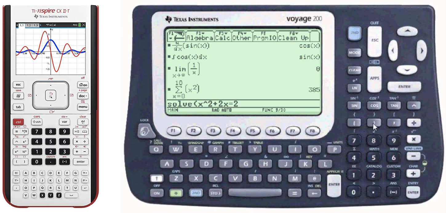
As human, we use symbols to carry out computations analytically. This can also be realized on computers using symbolic computation. There are many so called computer algebra systems (CAS) out there and you might already be familiar with one from school, if you have used a graphing calculator there like the ones shown below.
But of course CAS are not limited to external devices but also available as software for normal computers. The most commonly used computer algebra systems are Mathematica and SageMath/SymPy. We will use Sympy in this course because it is open-source and a Python library compared to Mathematica. SageMath is based on Sympy and offers a number of additional functionalities, which we do not need in this class.
SymPy can be installed by executing:
conda install -c anaconda sympy
To illustrate the difference between numerical and symbolic computations,
we compare the output of square root functions from numpy and sympy.
The code
import numpy as np
print(np.sqrt(8))
produces 2.8284271247461903 as output, which is an approximation to the
true value of (\sqrt(8)), while
import sympy as sp
print(sp.sqrt(8))
produces 2*sqrt(2), which is exact.
Basic Operations
We strongly advise you to try out the following small code examples yourself, preferably in a Jupyter notebook. There you can easily see the value of the variables and the equations can be rendered as latex. Just write the SymPy variable at the end of Jupyter cell without calling the
Defining Variables
Before solving any problem, we start defining our symbolic variables.
SymPy provides the constructor sp.Symbol() for this:
x = sp.Symbol('x')
This defines the Python variable x as a SymPy Symbol with the representation
'x'. If you print the variable in a Jupyter cell, you should see a rendered
symbol like: \( x \).
Since it might be annoying to define a lot variables, SymPy provides a another
function, which can initalizes a arbitrary number of symbols.
x, y, t, omega = sp.symbols('x y t omega')
which is just a shorthand for
x, y, t, omega = [sp.Symbol(n) for n in ('x', 'y', 't', 'omega')]
Note that it is important to separate each symbol in the sp.symbols() call
with a space.
SymPy also provides often used symbols (latin and greek letters) as predefined
variables. They are located in the submodule called abc
and can be imported by calling
from sympy.abc import x, y, nu
Expressions
Now we can use these variables to define an expression. We first want to define the following expression: $$ x + 2 y $$ SymPy allows us to write this expression in Python as we would do on paper:
x, y = sp.symbols('x y')
f = x + 2 * y
If you now print f in Jupyter cell you should see the same rendered equation
as above.
Lets assume we want to multiply our expression not by \( x \). We can
just do the following:
g = x * f
Now, we can print g and should get:
$$
x (x + 2y)
$$
One may expect this expression to transform into
\(x^2 + 2xy\), but we get the factorized form instead. SymPy
only performs obvious simplifications automatically, since one might
prefer the expanded of the factorized form depending on the circumstances.
But we can easily switch between both representations using the
transformation functions expand and factor:
g_expanded = sp.expand(g)
If you print g_expanded you should see, the expanded form of the equation, like:
$$
x^2 + 2xy
$$
Factorization of g_expanded brings us back to where we started.
g_factorized = sp.factor(g_expanded)
with the following representation: $$ x (x + 2y) $$
If you are feeling lazy, you can use the function simplify.
SymPy will then try to figure out which form would be the most suitable.
We can also write more complicated functions using elementary functions:
t, omega = sp.symbols('t omega')
f = sp.sqrt(2) / sp.sympify(2) * sp.exp(-t) * sp.cos(omega*t)
Note that since the division operator / on a number produces
floating-point numbers, we should modify numbers with the function sympify.
When dealing with rationals like 2/5, we can use sp.Rational(2, 5) instead.
If you print f the rendered equation should look like:
$$
\frac{\sqrt{2} e^{-t} \cos \left( \omega t \right)}{2}
$$
On some platforms, you may get a nicely rendered expression. While some
platform does not support nice printing, you could try to turn it on by
executing
sp.init_printing(use_unicode=True)
before any printing. We can also turn our expression into a function with either one
f_func1 = sp.Lambda(t, f)
or multiple arguments
f_func2 = sp.Lambda((t, omega), f)
by using the Lambda function. In the first case printing of f_func1
should look like
$$
\left(t \mapsto \frac{\sqrt{2} e^{-t} \cos (\omega t)}{2}\right)
$$
while f_func2 should give you:
$$
\left((t, \omega) \mapsto \frac{\sqrt{2} e^{-t} \cos (\omega t)}{2}\right)
$$
As you see these are still symbolic expressions, but the Python object is
now a callable function with either one or two positional arguments.
This allows us to substitute e.g. the variable \( t \) with
a number:
f_func1(1)
This gives us: $$ \frac{\sqrt{2} \cos (\omega)}{2 e} $$ We can also call our second function, which takes 2 arguments (\(t\), and \(\omega\)).
f_func2( sp.Rational(1, 2), 1 )
Which will result in:
$$
\frac{\sqrt{2} \cos \left(\frac{1}{2}\right)}{2 e^{\frac{1}{2}}}
$$
Note: We have now eliminated all variables and are left with an exact number, but this still
a SymPy object. You might wonder, how we can transform this to a numerical value which we can
use by other Python modules. SymPy provides this transformation with the function
lambdify, this looks similar to the Lambda function and also returns a Python function, that
we can call. However, the returned value of this function is now numerical value.
import math
f_num = sp.lambdify((t, omega), f)
assert math.isclose(f_num(0, 1), math.sqrt(2)/2)
Calculus
Calculus is hard. So why not let the computer do it for us?
Limits
Let us start by
evaluating the limit
$$\lim_{x\to 0} \frac{\sin(x)}{x}$$
We first define our variable \( x \) and the expression inside on the
right hand side. Then we can use the method limit to evaluate the
limit for \( x \to 0 \).
x = sp.symbols('x')
f = sp.sin(x) / x
lim = sp.limit(f, x, 0)
assert lim == sp.sympify(1)
Even one-sided limits like $$ \lim_{x\to 0^+} \frac{1}{x} \mathrm{\ \ vs.\ } \lim_{x\to 0^-} \frac{1}{x} $$ can be evaluated.
f = sp.sympify(1) / x
rlim = sp.limit(f, x, 0, '+')
assert rlim == sp.oo

llim = sp.limit(f, x, 0, '-')
assert llim == -sp.oo
Derivatives
Suppose we want find the first derivative of the following function
$$f(x, y) = x^3 + y^3 + \cos(x \cdot y) + \exp(x^2 + y^2)$$
We first start by defining the expression on the right side. In the next
step we can call the diff function, which expects an expression as the
first argument. The second to last argument (you can use one or more)
are the symbolic variables by which the expression will be derivated.
x, y = sp.symbols('x y')
f = x**3 + y**3 + sp.cos(x * y) + sp.exp(x**2 + y**2)
f1 = sp.diff(f, x)
In this we create the first derivative of \( f(x, y) \) w.r.t \(x\). You should get: $$ x^{3}+y^{3}+e^{x^{2}+y^{2}}+\cos (x y) $$
We can also build the second and third derivative w.r.t. x:
f2 = sp.diff(f, x, x)
f3 = sp.diff(f, (x, 3))
Note that two ways of computing higher derivatives are presented here. Of course, it is also possible to create the first derivative w.r.t \( x\) and \(y\):
f4 = sp.diff(f, x, y)
Evaluating Derivatives (or any other expression)
Sometimes, we want to evaluate derivatives, or just any expression at
specified points. For this purpose, we could again use Lambda to convert
the expression into a function and inserting values by function calls. But
SymPy expressions have the subs method to avoid the detour:
f = x**3 + y**3 + sp.cos(x*y) + sp.exp(x**2 + y**2)
f3 = sp.diff(f, (x, 3))
g = f3.subs(y, 0)
h = f3.subs(y, x)
i = f3.subs(y, sp.exp(x))
j = f3.subs([(x, 1), (y, 0)])
This method takes a pair of arguments. The first one is the variable to be substituted and the second one the value. Note that the value can also be a variable or an expression. A list of such pairs can also be supplied to substitute multiple variables.
Integrals
Even the most challenging part in calculus (integrals) can be evaluated $$ \int \mathrm{e}^{-x} \mathrm{d}x $$
f = sp.exp(-x)
f_int = sp.integrate(f, x)
This evaluates to $$ -e^{-x} $$ Note SymPy does not include the constant of integration. But this can be added easily by oneself if needed.
A definite integral could be computed by substituting the integration variable
with upper and lower bounds using subs. But it is more straightforward to
just pass a tuple as the second argument to the integrate function:
Suppose we want to compute the definite integral
$$\int_{0}^{\infty} \mathrm{e}^{-x}\ \mathrm{d}x$$
one can write
f = sp.exp(-x)
f_dint = sp.integrate(f, (x, 0, sp.oo))
assert f_dint == sp.sympify(1)
which evaluates to 1.
Also multivariable integrals like $$ \int_{-\infty}^{\infty} \int_{-\infty}^{\infty} \mathrm{e}^{-x^2-y^2}\ \mathrm{d}x \mathrm{d}y $$ can be easily solved. In this case the integral
f = sp.exp(-x**2 - y**2)
f_dint = sp.integrate(f, (x, -sp.oo, sp.oo), (y, -sp.oo, sp.oo))
assert f_dint == sp.pi
evaluates to \( \pi \).
Application: Hydrogen Atom
We learned in the bachelor quantum mechanics class that the wavefunction of the hydrogen atom has the following form: $$ \psi_{nlm}(\mathbf{r})=\psi(r, \theta, \phi)=R_{n l}(r) Y_{l m}(\theta, \phi) $$ where \(R_{n l}(r) \) is the radial function and \(Y_{l m}\) are the spherical harmonics. The radial functions are given by $$ R_{n l}(r)=\sqrt{\left(\frac{2}{n a}\right)^{3} \frac{(n-l-1) !}{2 n[(n+l) !]}} e^{-r / n a}\left(\frac{2 r}{n a}\right)^{l}\left[L_{n-l-1}^{2 l+1}(2 r / n a)\right] $$ Here \(n, l\) are the principal and azimuthal quantum number. The Bohr radius is denoted by \( a\) and \( L_{n-l-1}^{2l+1} \) is the associated/generalized Laguerre polynomial of degree \( n - l -1\). We will work with atomic units in the following, so that \( a = 1\). With this we start by defining the radial function:
def radial(n, l, r):
    n, l, r = sp.sympify(n), sp.sympify(l), sp.sympify(r)
    n_r = n - l - 1
    r0 = sp.sympify(2) * r / n
    c0 = (sp.sympify(2)/(n))**3
    c1 = sp.factorial(n_r) / (sp.sympify(2) * n * sp.factorial(n + l))
    c = sp.sqrt(c0 * c1)
    lag = sp.assoc_laguerre(n_r, 2 * l + 1, r0)
    return c * r0**l * lag * sp.exp(-r0/2)
We can check if we have no typo in this function by simply calling it with the three symbols
n, l, r = sp.symbols('n l r')
radial(n, l, r)
In the next step we can define the wave function by building the product of the radial function and the spherical harmonics.
from sympy.functions.special.spherical_harmonics import Ynm

def wavefunction(n, l, m, r, theta, phi):
    return radial(n, l, r) * Ynm(l, m, theta, phi).expand(func=True)
With this we have everything we need and we can start playing with wave functions of the Hydrogen atom. Let us begin with the simplest one, the 1s function \( \psi_{100} \).
n, l, m, r, theta, phi = sp.symbols('n l m r theta phi')
psi_100 = wavefunction(1, 0, 0, r, theta, phi)
We can now use what we learned in the previous chapter and evaluate for example the wavefunction in the limit of \(\infty\) $$ \lim_{r\to \infty} \psi_{100}(r, \theta, \phi) $$
psi_100_to_infty = sp.limit(psi_100, r, sp.oo)
assert psi_100_to_infty == sp.sympify(0)
This evaluates to zero, as we would expect. Now let's check if our normalization of the wave function is correct. For this we expect, that the following holds: $$ \int_{0}^{+\infty} \mathrm{d}r \int_{0}^{\pi} \mathrm{d}\theta \int_{0}^{2\pi} \mathrm{d}\phi \ r^2 \sin(\theta)\ \left| \psi_{100}(r,\theta,\phi) \right|^2 = 1 $$ We can easily check this, since we already learned how to calculate definite integrals.
dr = (r, 0, sp.oo)
dtheta = (theta, 0, sp.pi)
dphi = (phi, 0, 2*sp.pi)
norm = sp.integrate(r**2 * sp.sin(theta) * sp.Abs(psi_100)**2, dr, dtheta, dphi)
assert norm == sp.sympify(1)
Visualizing the wave functions of the H atom.
To visualize the wave functions we need to evaluate them on a finite grid.
Radial part of wave function.
For this example we will take a look at radial part of the first 4 s-functions. We start by defining them:
r = sp.symbols('r')
r10 = sp.lambdify(r, radial(1, 0, r))
r20 = sp.lambdify(r, radial(2, 0, r))
r30 = sp.lambdify(r, radial(3, 0, r))
r40 = sp.lambdify(r, radial(4, 0, r))
This gives us 4 functions that will return numeric values of the radial part at some radius \(r\). The radial electron probability is given by \(r^2 |R(r)|^2\). We will use these functions to evaluate the wave functions on a grid and plot the values with Matplotlib.
import matplotlib.pyplot as plt

r0 = 0
r1 = 35
N = 1000
r_values = np.linspace(r0, r1, N)
fig, ax = plt.subplots(1, 1, figsize=(8, 5))
ax.plot(r_values, r_values**2*r10(r_values)**2, color="black", label="1s")
ax.plot(r_values, r_values**2*r20(r_values)**2, color="red", label="2s")
ax.plot(r_values, r_values**2*r30(r_values)**2, color="blue", label="3s")
ax.plot(r_values, r_values**2*r40(r_values)**2, color="green", label="4s")
ax.set_xlim([r0, r1])
ax.legend()
ax.set_xlabel(r"distance from nucleus ($r/a_0$)")
ax.set_ylabel(r"electron probability ($r^2 |R(r)|^2$)")
fig.show()

Spherical Harmonics
In the next step, we want to graph the spherical harmonics. To do
this, we first import all the necessary modules and then define first the
symbolic spherical harmoncis, Ylm_sym and then the numerical function Ylm.
from sympy.functions.special.spherical_harmonics import Ynm
import sympy as sp
import numpy as np
import matplotlib.pyplot as plt
from matplotlib import cm
%config InlineBackend.figure_formats = ['svg']

l, m, theta, phi = sp.symbols("l m theta phi")
Ylm_sym = Ynm(l, m, theta, phi).expand(func=True)

Ylm = sp.lambdify((l, m, theta, phi), Ylm_sym)
The variable Ylm now contains a Python function with 4 arguments (l, m,
theta, phi) and returns the numeric value (complex number, type: complex)
of the spherical harmonics. To be able to display the function graphically,
however, we have to evaluate the function not only at one point, but on a
two-dimensional grid (\(\theta, \phi\)) and then display the values on this
grid. Therefore, we define the grid for \(\theta\) and \(\phi\) and evaluate
the \(Y_{lm} \) for each point on this grid.
N = 1000
theta = np.linspace(0, np.pi, N)
phi = np.linspace(0, 2*np.pi, N)
theta, phi = np.meshgrid(theta, phi)

l = 3
m = 0
Ylm_num = 1/2 * abs(Ylm(l, m, theta, phi) + Ylm(l, -m, theta, phi))
Now, however, we still have a small problem because we want to represent our data points in a Cartesian coordinate system, but our grid points are defined in spherical coordinates. Therefore it is necessary to transform the calculated values of Ylm into the Cartesian coordinate system. The transformation reads:
x = np.cos(phi) * np.sin(theta) * Ylm_num
y = np.sin(phi) * np.sin(theta) * Ylm_num
z = np.cos(theta) * Ylm_num
Now we have everything we need to represent the spherical harmonics in 3
dimensions. We do a little trick and map the data points to a number range from
0 to 1 and store these values in the variable colors. This allows us to
colorize the spherical harmonics with a colormap
from Matplotlib.
colors = Ylm_num / (Ylm_num.max() - Ylm_num.min())

fig = plt.figure(figsize=(10, 10))
ax = fig.add_subplot(111, projection="3d")

ax.plot_surface(x, y, z, facecolors=cm.seismic(colors))

ax.set_xlim([-1, 1])
ax.set_ylim([-1, 1])
ax.set_zlim([-1, 1])
fig.show()
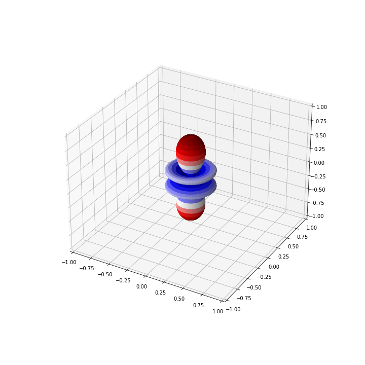
For the above example with \( Y_{30}\), the graph should look like
Application: Harmonic Oscillator
The quantum harmonic oscillator is described by wavefunctions $$ \psi_{n}(x) = \frac{1}{\sqrt{2^n n!}} \left( \frac{m \omega}{\pi \hbar} \right)^{1/4} \exp\left(-\frac{m\omega x^2}{2\hbar}\right) H_{n}\left( \sqrt{\frac{m\omega}{\hbar}} x \right) $$ where the functions \(H_{n}(z)\) are the physicists' Hermite polynomials: $$ H_{n}(z) = (-1)^n\ \mathrm{e}^{z^2} \frac{\mathrm{d}^n}{\mathrm{d}z^n} \left( \mathrm{e}^{-z^2} \right) $$ The corresponding energy levels are $$ E_{n} = \omega \left( n + \frac{1}{2} \right) $$
We now want to use SymPy to compute eigenenergies and eigenfunctions.
We start by importing sympy and neccesary variables:
import sympy as sp
from sympy.abc import x, m, omega, n, z
The eigenenergies are stright-forward to compute. One can just use the definition directly and substitute \(n\) by an integer, e.g. 5:
def energy(n):
    e = omega * (n + sp.Rational(1, 2))
    return e

e_5 = energy(5)
This outputs \(\frac{11}{2}\). Note that atomic units are used for simplicity.
In order to evaluate the wave function, we have to at first compute the Hermite polynomial. There are multiple ways to do it. The first is to use its definition directly and compute higher order derivatives of the exponential function:
def hermite_direct(n):
    h_n = (-1)**n * sp.exp(z**2) * sp.diff(sp.exp(-z**2), (z, n))
    h_n = sp.simplify(h_n)
    return h_n
Another way is to use the recurrence relation $$ H_{n+1}(z) = 2zH_{n}(z) - H_{n}^{'}(z) $$ which can be implemented as a recursive function:
def hermite_recursive(n):
    if n == 0:
        return sp.sympify(1)
    else:
        return sp.simplify(
            2 * x * hermite_recursive(n - 1) \
            - sp.diff(hermite_recursive(n - 1), x)
        )
For n = 5, both methods lead to the polynomial
$$ H_5(x) = 32 x^5 - 160 x^3 + 120 x$$
We can then use this to evaluate the wave function:
def wfn(n):
    nf = (1/sp.sqrt(2**n * sp.factorial(n))) \
         * ((m*omega)/sp.pi)**sp.Rational(1, 4)
    expf = sp.exp(-(m*omega*x**2)/2)
    hp = hermite_direct(n).subs(z, sp.sqrt(m*omega)*x)
    psi_n = sp.simplify(nf * expf * hp)

    return psi_n

psi_5 = wfn(5)
For a system with, say, \(m = 1\) and \(\omega = 1\), we can construct its wave function by
psi_5_param = psi_5.subs([(m, 1), (omega, 1)])
Further substituting x with any numerical value would evaluate the
wave function at that point. With the evalf method, we can obtain the
approximated numerical value:
psi_5_param_x_eval = psi_5_param.evalf(subs={x: sp.Rational(1, 2)})
print(psi_5_param_x_eval)
print(type(psi_5_param_x_eval))
Here, we compute the value of the wave function at \(x = \frac{1}{2}\).
We get 0.438575095003232 as the result. Note that the type of this object
is not float, but sympy.core.numbers.Float, which is a floating-point
number implementation with arbitrary precision. Actually, we can pass an
additional argument n to evalf to get an accuracy of n digits:
The listing
print(psi_5_param.evalf(n=50, subs={x: sp.Rational(1, 2)}))
for example, produces 0.43857509500323214478874587638315301825689754260515.
This type can be easily converted to python's built-in float by calling
float(). The arbitrary precision however, will be lost.
Sometimes one might just want to use SymPy to generate symbolic expressions
to be used in functions. Instead of typing the results in by hand, one could
use one of SymPy's built-in printers. Here, we shall use NumPyPrinter,
which converts a SymPy expression to a string of python code:
from sympy.printing.pycode import NumPyPrinter
printer = NumPyPrinter()
code = printer.doprint(psi_5_param)
code = code.replace('numpy', 'np')
print(code)
This output can be copied and used to evaluate \(\psi_{5}(x)\).
Since we often import NumPy with the alias np, numpy from the original
string is replaced.
Application: Particle in a Box
Problem
Determine the varianz und standard deviation for the location (\(x\)) and the momentum (\(p\)) for a particle in a box with a length of \(a\). Verify Heisenberg's uncertainty principle on this model.
The wave functions of a particle in a box is given by $$\psi_{n} = N \cdot \sin \left( \frac{n \pi}{a} x \right);\quad n \in \mathbb{N}$$ The variance of a quantity \(A\) is defined as $$\sigma_{A}^2 = \langle A^2 \rangle - \langle A \rangle^2$$
Solution
First, we import SymPy and define symbols with all necessary assumptions.
import sympy as sp
from sympy.physics.quantum.constants import hbar

x, N = sp.symbols('x N')
a = sp.Symbol('a', positive=True)
n = sp.Symbol('n', integer=True, positive=True)
(a) Define a function which performs integrals over \(x\) on the correct interval.
def integrate(expr):
    return sp.integrate(expr, (x, 0, a))
(b) Find the normalization constant \(N\).
wf = N * sp.sin((n*sp.pi/a) * x)
norm = integrate(wf**2)
N_e = sp.solve(sp.Eq(norm, 1), N)[1]
The constant N_e should evaluate to \(\sqrt{2/a}\).
(c) Define the wave function \(\psi_{n}\).
psi = N_e * sp.sin((n*sp.pi/a) * x)
(d) Determine \(\sigma_{x}\).
x_mean = integrate(sp.conjugate(psi) * x * psi)
x_mean = sp.simplify(x_mean)
x_rms = integrate(sp.conjugate(psi) * x**2 * psi)
x_rms = sp.simplify(x_rms)

var_x = x_rms - x_mean**2
sigma_x = sp.sqrt(var_x)
The expectation value of \(x\) evaluates to $$ \langle x \rangle = \frac{a}{2} $$ and that of \(x^2\) evaluates to $$ \langle x^2 \rangle = \frac{a^2}{3} - \frac{a^2}{2 \pi^2 n^2}$$ The standard deviation of \(x\) is thus $$ \sigma_{x} = \sqrt{ \frac{a^2}{12} - \frac{a^2}{2 \pi^2 n^2} } $$
(e) Determine \(\sigma_{p}\).
p_mean = integrate(sp.conjugate(psi) * (-sp.I*hbar) * sp.diff(psi, x))
p_mean = sp.simplify(p_mean)
p_rms = integrate(sp.conjugate(psi) * (-sp.I*hbar)**2 * sp.diff(psi, x, x))
p_rms = sp.simplify(p_rms)

var_p = p_rms - p_mean**2
sigma_p = sp.sqrt(var_p)
The expectation value of \(p\) equals to \(0\) while that of \(p^2\) is $$ \langle p^2 \rangle = \frac{\pi^2 n^2}{a^2} $$ The standard deviation of \(p\) is therefore $$ \sigma_{p} = \frac{\pi n}{a} $$
(f) Compute the product \(\sigma_{x} \cdot \sigma_{p}\).
product = sigma_x * sigma_p
product = sp.simplify(prod)
p1 = prod.subs(n, 1)
This product equals to $$ \sigma_{x} \cdot \sigma_{p} = \frac{\sqrt{3 \pi^2 n^2 - 18}}{6} $$
For \(n = 1\), this expression takes on the value \( \frac{\sqrt{3\pi^2 - 18}}{6} \), which is approximately \(0.568\). For larger \(n\)'s, its value becomes larger. Therefore, Heisenberg's uncertainly principle holds for the particle in a box model.
Fourier Transformation
Let us consider periodic function with some period \(L>0\). Due to the fact that any linear combination of two periodic function with the same period is again a periodic function, the space of the periodic functions is mathematically a vector space. It is thus natural to seek for a basis in the space of periodic functions.
The archetypical periodic functions are the sine and cosine functions, that can be together compactly represented in the form of a complex exponential:
$$\varphi(x)=\exp(\mathrm{i}kx),$$
where \(k\) is some real parameter.
If we now impose the periodicity with the period \(L\) on the complex exponential we obtain the following relation which restricts the possible values of \(k\):
$$\varphi(x+L)=\varphi(x)\rightarrow\exp(\mathrm{i}kL)=1.$$
This relation will be full filled only for a discrete set of \(k-\)values that are defined by the relation:
$$k_{n}L=2\pi n\quad n\in\mathbb{Z}.$$
In this a discrete set of complex exponential functions all with the fundamental period of \(L\) can be constructed:
$$\varphi_{n}(x)=\exp\left(\frac{\mathrm{i} 2\pi n}{L}x\right)\quad n\in\mathbb{Z}$$
from ipywidgets import interact
import ipywidgets as widgets
L = 1.0

def plot_exp(n):
    x = np.linspace(0, L, 500)
    y= np.exp(2.0j*np.pi*n*x/L)
    plt.xlim((-0.25, 1.25))
    plt.plot(x, y.real, lw = 3.0)
    plt.plot(x, y.imag, lw = 3.0)

interact(plot_exp, n=widgets.IntSlider(value=1, min=1, max=10, step=1))
The plot for \(n = 3\) is shown here:

Orthogonality of complex exponentials
We now show that the above defined periodic complex exponential constitute an orthonormal set of functions.
For this purpose we recall the definition of the complex inner product for two functions on an arbitrary interval [\(a,b\)], which is defined as:
$$ \langle f|g\rangle =\int_{a}^b \mathrm{d}x \ f^{ * } (x)g(x) $$
For two complex exponentials with indices \(m\) and \(n\) we have:
$$ \langle\varphi_{m}|\varphi_{n}\rangle=\int_{0}^{L} \mathrm{d}x \exp \left( \mathrm{i} \frac{2\pi}{L}(n-m)x \right) = \begin{cases} L & m=n \\ 0 & m \ne n \end{cases} $$
This can be compactly represented by introducing the Kronecker delta symbol:
$$\langle\varphi_{m}|\varphi_{n}\rangle=L\delta_{mn}$$
Thus, we now have a discrete set of orthonormal functions that can serve as a basis for representing arbitrary periodic function! The functions \(\varphi_{n}(x)\) are also called trigonometric polynomials since they can be expressed as:
$$\varphi_{n}(z)=z^{n}$$
Here \(z\) is a complex variable defined as:
$$z=\exp\left(\mathrm{i}\frac{2\pi x}{L}\right)$$
Approximating function by trigonometric polynomials
In the previous slide we have introduced the trigonometric polynomials. Now we introduce a formal definition. The function:
$$ \phi_{N}(x)=\sum_{j=0}^{N-1}c_{j}\exp\left(\mathrm{i}\frac{2\pi j}{L}x\right)$$
is called a trigonometric polynomial of the \(N-1\)-th order. The \(N-\)dimensional space of complex trigonometric polynomials is denoted by \(\mathbf{T}_ {N}^C \).
Let us now assume that we want to approximate some periodic function by a trigonometric polynomial of a degree \(N-1\). The problem consists in calculating the values of the expansion coefficients \(c_{j}\) that minimize the deviation between the two functions within a single period. In order to do this we have to define the distance between the two functions!
The metric in the function space is introduced in analogy to the distance between two vectors with discrete components and can be defined as:
$$d(f,g)=|\langle f-g|f-g\rangle|^{2}=\int_{0}^{L}\mathrm{d}x\ (f-g)^{ * }(f-g)$$
or
$$d(f,g)=|\langle f|f\rangle|^{2}+|\langle g|g\rangle|^{2}-\langle f|g\rangle-\langle g|f\rangle$$
Now, if we want to approximate the function \(f(x)\) by a trigonometric polynomials \(\phi_{N}(x)\) we have to minimize the distance between these two functions with respect to the coefficients of the trigonometric polynomial. The distance is given by:
$$d(f,\phi_{N})=|\langle f|f\rangle|^{2}+|\langle \phi_{N}|\phi_{N}\rangle|^{2}-\langle f|\phi_{N}\rangle-\langle \phi_{N}|f\rangle$$
The norm of the trigonometric polynom \(\langle \phi_{N}|\phi_{N}\rangle|^{2}\) can be calculated as:
$$ \langle\phi_{N}|\phi_{N}\rangle=\sum_{k=0}^{N-1}\sum_{j=0}^{N-1}c_{k}^{\ast}c_{j}\langle\varphi_{k}|\varphi_{j}\rangle=\sum_{k=0}^{N-1}\sum_{j=0}^{N-1}c_{k}^{\ast}c_{j}\delta_{kj}L $$
$$ \langle\phi_{N}|\phi_{N}\rangle=\sum_{j=0}^{N-1}c_{j}^{ * } c_{j}L = \sum_{j=0}^{N-1}|c_{j}|^2L $$
The remaining two scalar products can be expanded into:
$$\langle f|\phi_{N}\rangle=\sum_{j=0}^{N-1}c_{j}\langle f|\varphi_{n}\rangle$$
$$\langle\phi_{N}|f\rangle=\sum_{j=0}^{N-1}c_{j}^{ * }\langle\varphi_{n}|f\rangle$$
After inserting into the distance expression the latter turns into a multivariable function \(d(c_{1},\cdots,c_{N}) \):
$$ d(f,\phi_{N})\rightarrow d(c_{1},\cdots,c_{N})=|\langle f|f\rangle|^{2}+\left[\sum_{j=0}^{N-1}c_{j}^{\ast}c_{j}L-c_{j}\langle f|\varphi_{n}\rangle-c_{j}^{\ast}\langle\varphi_{n}|f\rangle\right] $$
This function is dependent on \(c_{j}\) and its complex conjugate \(c_{j}^{ * }\), which can be considered as two independent variables (equivalently we could treat their real and imaginary parts as independent variables!).
In order to minimize the distance we need to calculate the partial derivatives with respect to \(c_{j}\) and \(c_{j}^{ * }\) and set them to zero:
$$\frac{\partial d}{\partial c_{k}}=0\quad\mathrm{{and}}\quad\frac{\partial d}{\partial c_{k}^{ * }}=0,\qquad k=0,\cdots,N-1$$
This leads to the values of the expansion Fourier coefficients that provide the best approximation of a given function:
$$ c_{k} L - \langle \varphi_{k}|f \rangle=0 \rightarrow c_{k} = \frac{1}{L} \langle \varphi_{k} | f \rangle $$
$$ c_{k}^{\ast} L - \langle f | \varphi_{k} \rangle = 0 \rightarrow c_{k}^{\ast} = \frac{1}{L} \langle f | \varphi_{k} \rangle $$
Written out explicitly the Fourier coefficient reads:
$$c_{k}=\frac{1}{L}\langle\varphi_{k}|f\rangle=\frac{1}{L}\int_{0}^{L}\mathrm{d}x\ \varphi_{k}^{ * }(x)f(x)$$
$$ \require{color} \fcolorbox{red}{#f2d5d3}{ $c_{k}=\frac{1}{L}\int_{0}^{L}\mathrm{d}x\ f(x)\exp\left(-\mathrm{i}\frac{2\pi k}{L}x\right)$ } $$
Example 1
We consider the triangle (or hat) function defined as :
$$f(x)=1-|x|,\qquad-1\le x<1$$
In order to calculate the Fourier series approximation we use SymPy package.
import sympy as sp
from sympy.abc import x

triangle = 1 - abs(x)
fourier = sp.fourier_series(triangle, (x, -1, 1))
approx = []
norder = 10

for order in range(norder):
    approx.append(fourier.truncate(n=order))
    display(approx[-1])
Which gives us:
$$ 0 $$ $$ \frac{1}{2} $$ $$ \frac{4 \cos{\left(\pi x \right)}}{\pi^{2}} + \frac{1}{2} $$ $$ \frac{4 \cos{\left(\pi x \right)}}{\pi^{2}} + \frac{4 \cos{\left(3 \pi x \right)}}{9 \pi^{2}} + \frac{1}{2} $$ $$ \frac{4 \cos{\left(\pi x \right)}}{\pi^{2}} + \frac{4 \cos{\left(3 \pi x \right)}}{9 \pi^{2}} + \frac{4 \cos{\left(5 \pi x \right)}}{25 \pi^{2}} + \frac{1}{2} $$ $$ \frac{4 \cos{\left(\pi x \right)}}{\pi^{2}} + \frac{4 \cos{\left(3 \pi x \right)}}{9 \pi^{2}} + \frac{4 \cos{\left(5 \pi x \right)}}{25 \pi^{2}} + \frac{4 \cos{\left(7 \pi x \right)}}{49 \pi^{2}} + \frac{1}{2} $$ $$ \frac{4 \cos{\left(\pi x \right)}}{\pi^{2}} + \frac{4 \cos{\left(3 \pi x \right)}}{9 \pi^{2}} + \frac{4 \cos{\left(5 \pi x \right)}}{25 \pi^{2}} + \frac{4 \cos{\left(7 \pi x \right)}}{49 \pi^{2}} + \frac{4 \cos{\left(9 \pi x \right)}}{81 \pi^{2}} + \frac{1}{2} $$ $$ \frac{4 \cos{\left(\pi x \right)}}{\pi^{2}} + \frac{4 \cos{\left(3 \pi x \right)}}{9 \pi^{2}} + \frac{4 \cos{\left(5 \pi x \right)}}{25 \pi^{2}} + \frac{4 \cos{\left(7 \pi x \right)}}{49 \pi^{2}} + \frac{4 \cos{\left(9 \pi x \right)}}{81 \pi^{2}} + \frac{4 \cos{\left(11 \pi x \right)}}{121 \pi^{2}} + \frac{1}{2} $$ $$ \frac{4 \cos{\left(\pi x \right)}}{\pi^{2}} + \frac{4 \cos{\left(3 \pi x \right)}}{9 \pi^{2}} + \frac{4 \cos{\left(5 \pi x \right)}}{25 \pi^{2}} + \frac{4 \cos{\left(7 \pi x \right)}}{49 \pi^{2}} + \frac{4 \cos{\left(9 \pi x \right)}}{81 \pi^{2}} + \frac{4 \cos{\left(11 \pi x \right)}}{121 \pi^{2}} + \frac{4 \cos{\left(13 \pi x \right)}}{169 \pi^{2}} + \frac{1}{2} $$ $$ \frac{4 \cos{\left(\pi x \right)}}{\pi^{2}} + \frac{4 \cos{\left(3 \pi x \right)}}{9 \pi^{2}} + \frac{4 \cos{\left(5 \pi x \right)}}{25 \pi^{2}} + \frac{4 \cos{\left(7 \pi x \right)}}{49 \pi^{2}} + \frac{4 \cos{\left(9 \pi x \right)}}{81 \pi^{2}} + \frac{4 \cos{\left(11 \pi x \right)}}{121 \pi^{2}} + \frac{4 \cos{\left(13 \pi x \right)}}{169 \pi^{2}} + \frac{4 \cos{\left(15 \pi x \right)}}{225 \pi^{2}} + \frac{1}{2} $$
# uncomment the following line if you are using a Jupyter Notebook
#%config InlineBackend.figure_formats = ['svg']

s = sp.plot(triangle, (x, -1, 1),show = True, legend = False)
s[0].line_color = "red"

for series in approx:
    fs = sp.plot(series, (x, -1, 1), show=False, legend=False)
    fs[0].line_color = "black"
    s.append(fs[0])

s.show()


Example 2
As a second example we consider the step function defined as :
$$f(x)=\begin{cases} -1 & -1\le x<0 \\ +1 & 0\le x<1 \end{cases}$$
This function has a discontinuity at \( x = 0 \)!
We again use SymPy to analytically calculate its Fourier series.
hat = sp.Piecewise((-1, sp.Interval(-1,0).contains(x)),
                   (+1, sp.Interval(0,1).contains(x)))
fourier = sp.fourier_series(hat, (x, -1, 1))
approx = []
norder = 10

for order in range(norder):
    approx.append(fourier.truncate(n=order))
    display(approx[-1])
$$ 0 $$ $$ \frac{4 \sin{\left(\pi x \right)}}{\pi} $$ $$ \frac{4 \sin{\left(\pi x \right)}}{\pi} + \frac{4 \sin{\left(3 \pi x \right)}}{3 \pi} $$ $$ \frac{4 \sin{\left(\pi x \right)}}{\pi} + \frac{4 \sin{\left(3 \pi x \right)}}{3 \pi} + \frac{4 \sin{\left(5 \pi x \right)}}{5 \pi} $$ $$ \frac{4 \sin{\left(\pi x \right)}}{\pi} + \frac{4 \sin{\left(3 \pi x \right)}}{3 \pi} + \frac{4 \sin{\left(5 \pi x \right)}}{5 \pi} + \frac{4 \sin{\left(7 \pi x \right)}}{7 \pi} $$ $$ \frac{4 \sin{\left(\pi x \right)}}{\pi} + \frac{4 \sin{\left(3 \pi x \right)}}{3 \pi} + \frac{4 \sin{\left(5 \pi x \right)}}{5 \pi} + \frac{4 \sin{\left(7 \pi x \right)}}{7 \pi} + \frac{4 \sin{\left(9 \pi x \right)}}{9 \pi} $$ $$ \frac{4 \sin{\left(\pi x \right)}}{\pi} + \frac{4 \sin{\left(3 \pi x \right)}}{3 \pi} + \frac{4 \sin{\left(5 \pi x \right)}}{5 \pi} + \frac{4 \sin{\left(7 \pi x \right)}}{7 \pi} + \frac{4 \sin{\left(9 \pi x \right)}}{9 \pi} + \frac{4 \sin{\left(11 \pi x \right)}}{11 \pi} $$ $$ \frac{4 \sin{\left(\pi x \right)}}{\pi} + \frac{4 \sin{\left(3 \pi x \right)}}{3 \pi} + \frac{4 \sin{\left(5 \pi x \right)}}{5 \pi} + \frac{4 \sin{\left(7 \pi x \right)}}{7 \pi} + \frac{4 \sin{\left(9 \pi x \right)}}{9 \pi} + \frac{4 \sin{\left(11 \pi x \right)}}{11 \pi} + \frac{4 \sin{\left(13 \pi x \right)}}{13 \pi} $$ $$ \frac{4 \sin{\left(\pi x \right)}}{\pi} + \frac{4 \sin{\left(3 \pi x \right)}}{3 \pi} + \frac{4 \sin{\left(5 \pi x \right)}}{5 \pi} + \frac{4 \sin{\left(7 \pi x \right)}}{7 \pi} + \frac{4 \sin{\left(9 \pi x \right)}}{9 \pi} + \frac{4 \sin{\left(11 \pi x \right)}}{11 \pi} + \frac{4 \sin{\left(13 \pi x \right)}}{13 \pi} + \frac{4 \sin{\left(15 \pi x \right)}}{15 \pi} $$ $$ \frac{4 \sin{\left(\pi x \right)}}{\pi} + \frac{4 \sin{\left(3 \pi x \right)}}{3 \pi} + \frac{4 \sin{\left(5 \pi x \right)}}{5 \pi} + \frac{4 \sin{\left(7 \pi x \right)}}{7 \pi} + \frac{4 \sin{\left(9 \pi x \right)}}{9 \pi} + \frac{4 \sin{\left(11 \pi x \right)}}{11 \pi} + \frac{4 \sin{\left(13 \pi x \right)}}{13 \pi} + \frac{4 \sin{\left(15 \pi x \right)}}{15 \pi} + \frac{4 \sin{\left(17 \pi x \right)}}{17 \pi} $$
s = sp.plot(hat, (x, -1, 1), show=True, legend=False)
s[0].line_color = "red"

for series in approx:
    fs = sp.plot(series, (x, -1, 1),show = False, legend = False)
    fs[0].line_color = "black"
    s.append(fs[0])

s.show()


In these two numerical examples we have seen that both continous as well as discontinous functions can be approximated by Fourier series (trigonometric polynomials). In general the convergence of the Fourier series to a given function is assured if the following conditions named after Lejeune Dirichlet are fulfilled:
Dirichlet's conditions:
- \( f \) must be absolutely integrable over a period.
- \( f \) must be of bounded variation in any given bounded interval.
- \( f \) must have a finite number of discontinuities in any given bounded interval, and the discontinuities cannot be infinite.
Discrete and Fast Fourier Transformation
We have seen in the two above examples that for functions that are defined analytically the Fourier series can be in principle calculated exactly by analytic integration. For many practically interesting functions such integration cannot be performed explicitly. Moreover, functions are in practice often represented by discretely sampled values. For example, laboratory measurements produce discrete signals. Computers can also evaluate functions for a discrete set of numbers etc. In such cases we wish to compute the trigonometric polynomial approximation numerically.
Example: Audio data
Download trumpet.txt
Download piano.txt
import IPython.display as disp
import urllib.request

# Download trumpet.txt from the server
urllib.request.urlretrieve("http://codinginchemistry.com/trumpet.txt", "trumpet.txt")
# Download piano.txt from the server
urllib.request.urlretrieve("http://codinginchemistry.com/piano.txt", "piano.txt")

data_trumpet = np.loadtxt('trumpet.txt')
data_piano = np.loadtxt('piano.txt')
sampling_rate = 44100

plt.plot(data_trumpet[:3000])
plt.plot(data_piano[:3000])

display(disp.Audio(data_trumpet, rate=sampling_rate))
display(disp.Audio(data_piano, rate=sampling_rate))

Discrete Fourier Transformation (DFT)
In the following, we consider a periodic function that has been discretely sampled on an evenly distributed set of \(N\) sample points contained within a single period \(L\). Such points will have the coordinates:
$$ x_{k}=k\times\frac{L}{N}\qquad k=0,\cdots,N-1 $$
The trigonometric polynomial approximation evaluated at the sample points should reproduce the function values:
$$ f(x)=\sum_{j=0}^{N-1}F_{j}\exp\left(\mathrm{i}\frac{2\pi j}{L}x\right)\rightarrow f_{k}=\sum_{j=0}^{N-1}F_{j}\exp\left(\mathrm{i}\frac{2\pi j}{L}x_{k}\right) $$
This gives rise to the following relation between the function values at the sample points and the Fourier coefficients:
$$\require{color}$$ $$ \fcolorbox{red}{#f2d5d3}{ $f_{k}=\sum_{j=0}^{N-1}F_{j}\exp\left(\mathrm{i}\frac{2\pi jk}{N}\right)$ } $$
Which defines the Discrete Fourier Transformation (DFT)!
Our main task now it to numerically calculate Fourier coefficients \(F_{j}\) for a given set of discrete function values.
Before we proceed we introduce a shorthand notation that will make the expressions more transparent.
We introduce the shorthand notation for the complex \(N-\)th root of unity:
$$W_{N}=\exp\left[\frac{2\pi \mathrm{i}}{N}\right]$$
We furthermore define a matrix \(\mathbf M\) with elements:
$$ M_{kj} = W_{N}^{kj} = \exp\left[\frac{2\pi \mathrm{i} jk}{N}\right]. $$
Using this notation the discrete Fourier Transform can be written as:
$$ f_{k}=\sum_{j=0}^{N-1}M_{kj}F_{j} $$ which is nothing else than a matrix-vector product.
Thus the discrete Fourier transformation is a linear matrix transformation of a given vector or function values written compactly as:
$$\mathbf {f} = \mathbf {M}\mathbf {F}$$
The matrix transformation transforms the vector of Fourier coefficients \(\mathbf{F} \) into the vector of function values \( \mathbf{f} \) at the sample points!
In order to find the values of the Fourier coefficients we now have two distinct possibilities:
- Inverting the matrix \( \mathbf{M} \) such that the Fourier coefficients can be determined as \( \mathbf {F} = \mathbf {M}^{-1}\mathbf {f} \).
- Calculate Fourier coefficients by some discrete approximation for the integral $$ c_{k}=\frac{1}{L}\int_{0}^{L}\mathrm{d}x\ f(x)\exp\left(-\mathrm{i}\frac{2\pi k}{L}x\right) $$ We first follow the route 1 and prove by explicit calculation that the matrix \( \mathbf M \) is up to a constant of \( N \) unitary.
For this purpose we calculate a general matrix element as follows:
$$\mathbf{M}^{\dagger}\mathbf{M}=?$$
$$\left(\mathbf{M}^{\dagger}\mathbf{M}\right)_ {ij}=\sum_{k=0}^{N-1}\left(\mathbf{M}^{\dagger}\right)_ {ik}\left(\mathbf{M}\right)_ {kj}=\sum_{k=0}^{N-1}\left(W_{N}^{ * }\right)^{ik}W_{N}^{kj} $$
By exploiting properties of the complex roots of unity we can easily prove that:
$$(W_{N}^{ * })^{ik}=\left(W_{N}^{ik}\right)^{ * }=W_{N}^{-ik}$$
This can be utilized to rewrite the matrix element as:
$$\left(\mathbf{M}^{\dagger}\mathbf{M}\right)_ {ij}=\sum_{k=0}^{N-1}W_{N}^{k(j-i)}$$
We now consider two cases:
Case 1: \( i = j \):
$$\left(\mathbf{M}^{\dagger}\mathbf{M}\right)_ {ii}=\sum_{k=0}^{N-1}1=N$$
Case 2: \( i \ne j\):
$$\left(\mathbf{M}^{\dagger}\mathbf{M}\right)_ {ij}=\sum_{k=0}^{N-1}\left[W_{N}^{(j-i)}\right]^{k}=\frac{1-\left(W_{N}^{N}\right)^{j-i}}{1-W_{N}^{(j-i)}}=0$$
Here, we have utilized the formula for the partial sum of a geometric series as well as the following identity:
$$W_{N}^{N}=1$$
This shows that the matrix $\mathbf M$ has an inverse determined by the relation:
$$\mathbf{M}^{\dagger}\mathbf{M}=N\mathbf{I}\rightarrow \mathbf{M}^{-1}=\frac{1}{N}\mathbf{M}^{\dagger}$$
This can now be utilized in order to perform the discrete Fourier transformation and calculate the Fourier coefficients:
$$\mathbf{f}=\mathbf{M}\mathbf{F}\rightarrow\mathbf{F}=\mathbf{M}^{-1}\mathbf{f}=\frac{1}{N}\mathbf{M}^{\dagger}\mathbf{f}$$
Explicitly in terms of the input vector components the Fourier coefficients read:
$$\fcolorbox{red}{#f2d5d3} {$F_{k}=\frac{1}{N}\sum_{j=0}^{N-1}f_{j}\exp\left(-\mathrm{i}\frac{2\pi jk}{N}\right)$}$$
Together with the inverse relation:
$$ \fcolorbox{green}{#d3f2d9}{$ f_{k}=\sum_{j=0}^{N-1}F_{j}\exp\left(\mathrm{i}\frac{2\pi jk}{N}\right)$}$$
These expressions fully specify the discrete Fourier transformation and its inverse!
What if we would have followed the route 2 and calculate the Fourier coefficients by approximating the integral:
$$F_{k}=\frac{1}{L}\int_{0}^{L}\mathrm{d}x\ f(x)\exp\left(-\mathrm{i}\frac{2\pi k}{L}x\right)$$
using some of the numerical integration procedures (e. g. trapezoidal or Simpson's rule)?
Most numerical integration schemes can be recast in the following general from by introducing the integration weights for each sample point:
$$\int_{0}^{L}f(x)\mathrm{d}x=\frac{L}{N}\sum_{j=0}^{N-1}w_{j}f(x_{j})$$
If we now apply this to the Fourier coefficients we get:
$$ F_{k} = \frac{1}{L}\int_{-\frac{L}{2}}^{+\frac{L}{2}}\mathrm{d}x\ f(x)\exp\left(-\mathrm{i}\frac{2\pi k}{L}x\right) \rightarrow F_{k}\approx\frac{1}{N}\sum_{j=0}^{N-1}w_{j}f_{j}\exp\left(-\mathrm{i}\frac{2\pi jk}{N}\right). $$
Thus, different numerical integration schemes would generally lead to different Fourier coefficients.
If we choose all weights to be equal to one, which corresponds to the usual trapezoidal rule we recovere the Fourier coefficients that we have determined along the route 1 exploiting the unitarity of the \(\mathbf M\)-matrix!
The advantage of this choice in contrast to all other possible integration scheme is that in this way the values of the input function at the sample points are exactly recovered if the inverse transformation is performed. In order to show this let us calculate the value of the trigonometric polynomial at the point \(x_{i}\):
$$f(x_{i})=\sum_{k=0}^{N-1}F_{k}W_{N}^{ik}$$
By inserting the Fourier coefficient obtained by a general numerical integration scheme:
$$F_{k}=\frac{1}{N}\sum_{j=0}^{N-1}w_{j}f_{j}W_{N}^{-jk}$$
we get:
$$f(x_{i})=\frac{1}{N}\sum_{k=0}^{N-1}\sum_{j=0}^{N-1}w_{j}f_{j}W_{N}^{(i-j)k}$$
which results in the following value of the trigonometric polynomial at the sampling point \(x_i\):
$$f(x_{i})=\frac{1}{N}\sum_{j=0}^{N-1}w_{j}f_{j}\sum_{k=0}^{N-1}W_{N}^{(i-j)k}=\sum_{j=0}^{N-2}w_{j}f_{j}\delta_{ij} = w_{i} f_{i}$$
We see that only in the case where \(w_{i}=1\) the trigonometric interpolation will be exact at the sampling points.
$$f(x_{i})=f_{i}$$
Since we anyway do not know anything about the function between the sampling points it is reasonable to require from the interpolation scheme that it reproduces the exact values at the sampling points!
Rudimentary DFT implementation
def dft1(f):
    f = np.asarray(f)
    N = f.shape[0]
    W = np.exp(-2 * np.pi * 1.0j / N)
    F = np.zeros(f.shape, dtype=complex)
    for k in range(N):
        F[k] = 0.0
        Wk = W**k
        for j in range(N):
            F[k] += f[j] * (Wk**j)
    return F
f = data_piano[:2000]
F = dft1(f)
N = len(f)
dx = 1. / sampling_rate
freq = 1.0 / (N * dx) * np.arange(N)
plt.plot(freq[:100], F.real[:100])
F_numpy = np.fft.fft(f)
frequency_numpy = np.fft.fftfreq(N, dx)
print(np.allclose(F, F_numpy))
plt.plot(frequency_numpy[:100], F_numpy[:100].real)
Our algorithm dft1 as well as fft from NumPy give us the same result:

Computational scaling of DFT
Since the DFT can be formulated as a matrix-vector product, its brute force evaluation will require for each component the calculation of N products of two numbers and addition of \(N\) numbers. Thus, the cost of the DFT should scale with the square of the data dimension \(N\). In the following we check numerically the computational scaling by performing DFT on randomly generated vectors with increasing number of components.
import random

Ntest = 10
timings1 = []
dimension = []

for i in range(1, Ntest):
    f = [random.gauss(0, 1) for n in range(2**i)]
    timing = %timeit -o -n 1 dft1(f)
    dimension.append(2**i)
    timings1.append(timing.average)
plt.subplot(121)
plt.plot(np.array(dimension), np.array(timings1), 'o', markersize=12, color='red')
plt.plot(np.array(dimension), np.array(timings1), color='red')
plt.xlabel("$N$")
plt.ylabel("Timing / s")

plt.subplot(122)
plt.plot(np.array(dimension)**2, np.array(timings1), 'o', markersize=12, color='red')
plt.plot(np.array(dimension)**2, np.array(timings1), color='red')

plt.xlabel("$N^2$")
plt.show()

A fancier brute-force DFT implementation using NumPy features
def dft2(f):
    f = np.asarray(f)
    N = f.shape[0]
    W = np.exp(-2 * np.pi * 1.0j / N)
    k = np.arange(N)
    jk = np.outer(k, k)
    M = W**jk
    return np.dot(M, f)
f = data_piano[:2000]
F = dft2(f)
N = len(f)
dx = 1. / sampling_rate
freq = 1.0 / (N * dx) * np.arange(N)
plt.plot(freq[:100], F.real[:100])
F_numpy = np.fft.fft(f)
frequency_numpy = np.fft.fftfreq(N, dx)
print(np.allclose(F, F_numpy))
plt.plot(frequency_numpy[:100], F_numpy[:100].real)
Our algorithm dft2 also produces the same result as fft from NumPy.

Timing with size
import random

Ntest = 10
timings2 = []
dimension2 = []

for i in range(1, Ntest):
    f = [random.gauss(0, 1) for n in range(2**i)]
    timing = %timeit -o -n 1 dft2(f)
    dimension2.append(2**i)
    timings2.append(timing.average)
plt.subplot(121)
plt.plot(np.array(dimension2), np.array(timings2), 'o', markersize=12, color='red')
plt.plot(np.array(dimension2), np.array(timings2), color='red')
plt.xlabel("$N$")
plt.ylabel("Timing / s")

plt.subplot(122)
plt.plot(np.array(dimension2)**2, np.array(timings2), 'o', markersize=12, color='red')
plt.plot(np.array(dimension2)**2, np.array(timings2), color='red')

plt.xlabel("$N^2$")
plt.show()

Comparison between two implementations
plt.plot(np.array(dimension), np.array(timings1), 'o', markersize=12, color='red')
plt.plot(np.array(dimension), np.array(timings1), color='red')
plt.plot(np.array(dimension2), np.array(timings2), 'o', markersize=12, color='blue')
plt.plot(np.array(dimension2), np.array(timings2), color='blue')

plt.xlabel("$N$")
plt.ylabel("Timing / s")

Fast Fourier Transformation (FFT) algorithm
We have seen that the brute force implementation of the discrete Fourier transform scales with the square of the number of data (\(N^2\)) which makes Fourier transforming large data sets extremely time-consuming. However, there is a very clever trick first discovered by Gauss that allows to perform the discrete Fourier transformation much more efficiently and leads to the \( \mathcal{O}(N\times \log N)\) scaling.
The resulting algorithm is called Fast Fourier Transform (FFT) and is a basis for a tremendous number of technological and scientific approximations.
The FFT-algorithm is considered to be the most far-reaching algorithm in computing and has revolutionalized signal processing. Although originally introduced by Gauss who tried to calculate orbits of asteroid Juno, it was rediscovered in the 20th century by the American mathematicians Cooley and Tukey.
In the following, we develop and implement one variant of the Cooley-Tukey's algorithm.
We recall once more the definition of the discrete Fourier transform of a vector \(\mathbf{f}\) and rewrite it in a slightly modified form:
$$NF_{k}=\sum_{j=0}^{N-1}f_{j}W_{N}^{kj}\quad k=0,\cdots N-1$$
with
$$ W_{N}=\exp\left[-\frac{2\pi \mathrm{i}}{N}\right] $$
Most variants of the FFT-algorithm are formulated in the simplest way if we assume that the number of data points N is a power of two (\(N=2^{n}\)).
In this case, the above sum can be also rewritten by summing only over the first half of the summation indices such that:
$$ NF_{k}=\sum_{j=0}^{N/2-1}\left(f_{j}W_{N}^{kj}+f_{j+\frac{N}{2}}W_{N}^{\left(j+\frac{N}{2}\right)k}\right) $$
By utilizing the properties of the complex exponentials we can show that:
$$ W_{N}^{\left(k+\frac{N}{2}\right)j}=W_{N}^{kj}W_{N}^{\frac{N}{2}k} $$
Furthermore, $$ W_{N}^{\frac{N}{2}k}=\exp\left[-\frac{2\pi \mathrm{i}}{N}\times\frac{N}{2}\right]^{k}=\left(\exp(-\mathrm{i}\pi)\right)^{k}=(-1)^{k} $$
With this, we can rewrite the discrete Fourier transform as:
$$NF_{k}=\sum_{j=0}^{\frac{N}{2}-1}\left[f_{j}+(-1)^{k}f_{j+\frac{N}{2}}\right]W_{N}^{kj}$$
Now, it is natural to separate the Fourier coefficients into the ones with odd and even indices. With this, we can rewrite the discrete Fourier transform as:
$$NF_{l}^{e}=NF_{2l}=\sum_{j=0}^{\frac{N}{2}-1}\left[f_{j}+(-1)^{2l}f_{j+\frac{N}{2}}\right]W_{N}^{2lj}\quad l=1,\cdots\frac{N}{2}$$
$$NF_{l}^{o}=NF_{2l+1}=\sum_{j=0}^{\frac{N}{2}-1}\left[f_{j}+(-1)^{2l+1}f_{j+\frac{N}{2}}\right]W_{N}^{\left(2l+1\right)j}\quad l=1,\cdots\frac{N}{2}$$
By noting that: \(W_{N}^{2lj}=W_{N/2}^{lj}\) and \(W_{N}^{\left(2l+1\right)j}=W_{N/2}^{lj}W_{N}^{j}\)
we can further simplify the above expressions by introducing wo auxiliary arrays:
$$g_{j}=f_{j}+f_{j+\frac{N}{2}}\quad j=1,\cdots,\frac{N}{2}$$
$$h_{j}=\left[f_{j}-f_{j+\frac{N}{2}}\right]W_{N}^{j}\quad j=1,\cdots,\frac{N}{2}.$$
which gives us for the even and odd components of the Fourier coefficients the following expression:
$$NF_{l}^{e}= \sum_{j=0}^{\frac{N}{2}-1}g_{j}W_{N/2}^{lj}$$ $$NF_{l}^{o}= \sum_{j=0}^{\frac{N}{2}-1}h_{j}W_{N/2}^{lj}$$
The central observation now is to realize that these are just two new discrete Fourier transforms with half as many of the data points. This leads to a conceptually very simple recursive FFT-algorithm!
Decimation in frequency FFT (recursive implementation)
def fft_dif_recursive(f):
    f = np.asarray(f)
    N = f.shape[0]
    W = np.exp(-2. * np.pi * 1.0j / N)
    if N == 1:
        return f
    else:
        indrange = np.arange(N / 2)
        f1,f2 = f[:N // 2], f[N // 2:]
        f_even = f1 + f2
        f_odd = (f1 - f2) * (W**(indrange))
        F1 = fft_dif_recursive(f_even)
        F2 = fft_dif_recursive(f_odd)

        F = np.zeros(N, dtype=complex)
        indrange = np.arange(N)
        F[indrange[::2]] = F1
        F[indrange[1::2]] = F2
        return F
f = data_piano[:2000]
f = np.pad(f, 24)
F = fft_dif_recursive(f)
N = len(f)
dx = 1. / sampling_rate
freq = 1.0 / (N * dx) * np.arange(N)
plt.plot(freq[:100], F.real[:100])
F_numpy = np.fft.fft(f)
frequency_numpy = np.fft.fftfreq(N, dx)
print(np.allclose(F, F_numpy))
plt.plot(frequency_numpy[:100], F_numpy[:100].real)
Our implementation fft_dif_recursive as well as fft from Numpy
give us the same result:

Signal Analysis
import IPython.display as disp

def closestPowerOfTwo(n):
    n = n - 1
    while n & n - 1:
        n = n & n - 1
    return n << 1

ndata = data_trumpet.shape[0]
n2 = closestPowerOfTwo(ndata)
data_trumpet = np.pad(data_trumpet, (n2-ndata) // 2)
#plt.plot(data_trumpet)
display(disp.Audio(data_trumpet, rate=sampling_rate))

F = fft_dif_recursive(data_trumpet)
N = len(data_trumpet)
dx = 1. / sampling_rate
freq = 1.0 / (N * dx) * np.arange(N)

plt.plot(freq[:4000], np.abs(F)[:4000]**2)
F_numpy = np.fft.fft(data_trumpet)
freq_numpy = np.fft.fftfreq(N, dx)
plt.plot(freq_numpy[:10000], np.abs(F_numpy)[:10000]**2)

Numerical derivatives
def ifft_dif_recursive(f):
    f = np.asarray(f)
    N = f.shape[0]
    W = np.exp(2. * np.pi * 1.0j / N)
    if N == 1:
        return f
    else:
        indrange = np.arange(N // 2)
        f1,f2 = f[:N//2], f[N//2:]
        f_even = f1 + f2
        f_odd = (f1 - f2) * (W**(indrange))
        F1 = ifft_dif_recursive(f_even)
        F2 = ifft_dif_recursive(f_odd)

        F = np.zeros(N, dtype=complex)
        indrange = np.arange(N)
        F[indrange[::2]] = F1
        F[indrange[1::2]] = F2
        return F
def gauss(x):
    return np.exp(-x**2)
def dgauss(x):
    return -2*x*np.exp(-x**2)

x = np.linspace(-3, 3, 32)
y = gauss(x)
dy = dgauss(x)
N = x.shape[0]
dx = x[1] - x[0]

print(N)
plt.plot(x, y, color='red', lw=3)
plt.plot(x, dy, color='blue', lw=3)
plt.xlabel('x')
plt.ylabel('y(x)')

F = fft_dif_recursive(y)
freq = (2 * np.pi / N/ dx) * np.concatenate((np.arange(N // 2), np.arange(-N // 2, 0, 1)))
F = 1.0j * F * freq
dy2 = ifft_dif_recursive(F) / (N)
plt.plot(x, dy2.real, 'o')

Comparison with dft2
Ntest = 10
timings3 = []
dimension = []
for i in range(1, Ntest):
    f = [random.gauss(0, 1) for n in range(2**i)]
    timing = %timeit -o -n 1 fft_dif_recursive(f)
    dimension.append(2**i)
    timings3.append(timing.average)
plt.subplot(121)
plt.plot(np.array(dimension), np.array(timings3), 'o', markersize=12, color='red')
plt.plot(np.array(dimension), np.array(timings3), color = 'red')
plt.plot(np.array(dimension2), np.array(timings2), 'o', markersize=12, color='blue')
plt.plot(np.array(dimension2), np.array(timings2), color='blue')


plt.xlabel("$N$")
plt.ylabel("Timing / s")
plt.show()

Numerical Solution of SE using FFT
$$\require{color}$$
Our goal is to numerically exactly solve the 1D-Schrödinger equation with an arbitrary potential \( V(x) \).
As well known from the courses on quantum mechanics Schrödinger equation reads:
$$\hat{H}|\psi\rangle=E|\psi\rangle$$
Here, \( \hat H \) is a Hamiltonian consisting of a kinetic energy and potential energy operators:
$$\hat{H}=\frac{\hat{p}^{2}}{2m}+V(\hat{x})$$
so that the eigenproblem can be written as:
$$\left[\frac{\hat{p}^{2}}{2m}+V(\hat{x})\right]|\psi\rangle=E|\psi\rangle$$
or explicitly,
$$\frac{\hat{p}^{2}}{2m}|\psi\rangle+V(\hat{x})|\psi\rangle=E|\psi\rangle$$
So far, we do not use any particular basis but represent the state \( |\psi \rangle \) as an arbitrary vector in the Hilbert space. Now we will project the eigenproblem onto a continous position eigenstate basis \( |x\rangle \) giving rise to the position representation of the Schrödinger equation:
$$\langle x|\frac{\hat{p}^{2}}{2m}|\psi\rangle+\langle x|V(\hat{x})|\psi\rangle=E\langle x|\psi\rangle$$
In the first part of the left hand side we now have a kinetic energy operator acting on a state \( \psi \). Since the kinetic energy operator is a square of the momentum operator, the most natural way to calculate this expression is to turn into the momentum representation by using the completeness of the momentum operator eigenfunctions:
$$\mathbb{1} = \int_{-\infty}^{+\infty}\text{d}p |p\rangle \langle p| $$
By inserting the completeness relation between the kinetic energy operator and the state \(|\psi\rangle \) we obtain:
$$\frac{\hat{p}^{2}}{2m}|\psi\rangle=\int_{-\infty}^{+\infty}\text{d}p\frac{\hat{p}^{2}}{2m}|p\rangle\langle p|\psi\rangle,$$
which leads to:
$$\int_{-\infty}^{+\infty}\text{d}p\langle x|\frac{\hat{p}^{2}}{2m}|p\rangle \langle p|\psi\rangle+\langle x|V(\hat{x})|\psi\rangle=E\langle x|\psi\rangle.$$
Now we can exploit the fact that the momentum eigenstate is also an eigenstate of the kinetic energy operator,
$$ \frac{\hat{p}^{2}}{2m}|p\rangle=\frac{p^{2}}{2m}|p\rangle, $$
which leads to: $$\int_{-\infty}^{+\infty}\text{d}p\frac{p^{2}}{2m}\langle x|p\rangle \fcolorbox{red}{#f2d5d3}{$\langle p|\psi\rangle$}+\langle x|\fcolorbox{green}{#d3f2d9}{$V(\hat{x})|\psi\rangle$}=E\langle x|\psi\rangle.$$ The first highlighted expression is the momentum representation of the state \( |\psi\rangle \), which can be obtained from the position representation by inserting the completeness relation for the position eigenstates:
$$\fcolorbox{red}{#f2d5d3}{$\langle p|\psi\rangle$}=\int_{-\infty}^{+\infty}\text{d}x'\langle p|x'\rangle\langle x'|\psi\rangle.$$
The second highlighted expression can be further expanded by inserting the completeness relation for the position eigenstates between the potential operator and the state \( |\psi\rangle\):
$$\fcolorbox{green}{#d3f2d9}{$V(\hat{x})|\psi\rangle$}=\int_{-\infty}^{+\infty}\text{d}x'V(\hat{x})|x'\rangle\langle x'|\psi\rangle$$
By introducing these expressions into the Schrödinger equation and interchanging the order of integration we obtain:
$$\int_{-\infty}^{+\infty}\text{d}x'\int_{-\infty}^{+\infty}\text{d}p\frac{p^{2}}{2m}\langle x|p\rangle\langle p|x'\rangle\langle x'|\psi\rangle+\int_{-\infty}^{+\infty}\text{d}x'\langle x|V(\hat{x})|x'\rangle\langle x'|\psi\rangle=E\langle x|\psi\rangle$$
or
$$\int_{-\infty}^{+\infty}\text{d}x'\left[\int_{-\infty}^{+\infty}\text{d}p\frac{p^{2}}{2m}\langle x|p\rangle\langle p|x'\rangle+\langle x|V(\hat{x})|x'\rangle\right]\langle x'|\psi\rangle=E\langle x|\psi\rangle$$
We now introduce the following shorthand notation: $$\psi(x):=\langle x|\psi\rangle$$
$$\psi(x'):=\langle x'|\psi\rangle$$
$$H(x,x'):=\int_{-\infty}^{+\infty}\text{d}p\frac{p^{2}}{2m}\langle x|p\rangle\langle p|x'\rangle+\langle x|V(\hat{x})|x'\rangle$$
$$\int_{-\infty}^{+\infty}\text{d}x'H(x,x')\psi(x')=E\psi(x)$$
With this, we have converted the Schrödinger equation into an eigenvalue problem for a continous ''matrix'' \( H(x,x') \)! In the next step, we will discretize the continous position variables \(x\) and \(x'\) and turn the infinite dimensional eigenvalue problem for a continous matrix \(H(x,x')\) into a usual discrete eigenvalue problem for a finite dimensional matrix!
Discretization of the Schrödinger equation
$$\require{color}$$ The Hamiltonian matrix in the continous position state basis is given by:
$$H(x,x')=\int_{-\infty}^{+\infty}\text{d}p\frac{p^{2}}{2m}\langle x|p\rangle\langle p|x'\rangle+\langle x|V(\hat{x})|x'\rangle$$
From the quantum mechanics we know that the scalar product of the position and momentum eigenstates is given by:
$$\langle x|p\rangle=\frac{1}{\sqrt{2\pi\hbar}}\exp\left(\frac{\text{i}px}{\hbar}\right),$$
being nothing else but the position representation of a momentum eigenstate. By taking the complex conjugate one can also replace the second scalar product by:
$$\langle p|x'\rangle=\frac{1}{\sqrt{2\pi\hbar}}\exp\left(-\frac{\text{i}px'}{\hbar}\right)$$
Thus, the matrix element can be rewritten as:
$$H(x,x')=\frac{1}{2\pi\hbar}\int_{-\infty}^{+\infty}\text{d}p\frac{p^{2}}{2m}\exp\left(\frac{\text{i}p(x-x')}{\hbar}\right)+\langle x|V(\hat{x})|x'\rangle$$
Already here, we recognize a continous Fourier transform in the kinetic part of the hamiltonian expression!
We can now discretize this by introducing a grid in the position and the momentum space :
$$x_{i}=x_{min}+i\Delta x\qquad i=0,\cdots,N-1$$
$$p_{k}=p_{min}+k\Delta p\qquad k=0,\cdots N-1$$
In this way, the continous matrix \( H(x,x') \) is represented by a discrete matrix:
$$H(x,x')\rightarrow h_{ij}=\frac{1}{2\pi\hbar}\sum_{k=0}^{N-1}\Delta p\frac{p_{k}^{2}}{2m}\exp\left(\frac{\text{i}p_{k}(i-j)\Delta x}{\hbar}\right)+\frac{1}{\Delta x}V(x_{i})\delta_{ij}$$
Here, we have utilized the fact that:
$$\langle x|V(\hat{x})|x'\rangle = V(x)\langle x|x'\rangle = V(x)\delta(x-x')$$
which can be transformed into
$$\langle x|V(\hat{x})|x'\rangle\rightarrow\langle x_{i}|V(\hat{x})|x_{j}\rangle=V(x_{i})\delta\left[(i-j)\Delta x\right]=\frac{1}{\Delta x}V(x_{i})\delta_{ij}$$
by utilizing the scaling property of the Dirac's delta function:
$$\delta (\alpha x)={\frac {\delta (x)}{|\alpha |}}.$$
By utilizing the positon space grid, the continous version of the eigenvalue problem can be turned into:
$$\begin{array}{c} \int_{-\infty}^{+\infty}\text{d}x'H(x,x')\psi(x')=E\psi(x)\\ \downarrow \end{array}$$
$$\sum_{j=1}^{N-1}\left[\sum_{k=0}^{N-1}\frac{\Delta x\Delta p}{2\pi\hbar}\frac{p_{k}^{2}}{2m}\exp\left(\frac{\text{i}p_{k}(i-j)\Delta x}{\hbar}\right)+V(x_{i})\delta_{ij}\right]\psi_{j}=E\psi_{i}\quad i=0,\cdots,N-1$$
where \( \psi_{i} :=\psi(x_{i}) \) and \( \psi_{j} :=\psi(x_{j}) \) has been introduced as a shorthand notation.
This now represents an usual matrix eigenvalue problem:
$$\sum_{j=0}^{N-1}H_{ij}\psi_{j}=E\psi_{i}\quad i=0,\cdots,N-1,$$
with hamiltonian matrix elements defined by:
$$H_{ij}=\sum_{k=0}^{N-1}\frac{\Delta x\Delta p}{2\pi\hbar}\frac{p_{k}^{2}}{2m}\exp\left(\frac{\text{i}p_{k}(i-j)\Delta x}{\hbar}\right)+V(x_{i})\delta_{ij}$$
In order to finish the discretization, we will now transform the hamiltonian matrix elements in a shape that will allow us to calculate them using standard Fast-Fourier-Transform (FFT) routine, which is available in the numpy.fft package.
We recall that:
$$ p_{k}=p_{min}+k\Delta p\quad k=0,\cdots,N-1 $$
This can be inserted into the expression for the matrix element: $$H_{lj}=\sum_{k=0}^{N-1}\frac{\Delta x\Delta p}{2\pi\hbar}\frac{\left[p_{min}+k\Delta p\right]^{2}}{2m}\exp\left(\frac{\text{i}(p_{min}+k\Delta p)(i-j)\Delta x}{\hbar}\right)+V(x_{i})\delta_{ij}$$
and can be simplified to:
$$H_{ij}=\exp\left(\frac{\text{i}(p_{min}(i-j)\Delta x}{\hbar}\right)\sum_{k=0}^{N-1}\frac{\Delta x\Delta p}{2\pi\hbar}\frac{\left[p_{min}+k\Delta p\right]^{2}}{2m}\exp\left(\frac{\text{i}k(i-j)\Delta x\Delta p}{\hbar}\right)+V(x_{i})\delta_{ij}$$
Since the integration range in the momentum space has to be symmetric, the lowest and the highest value of the discretized momentum need to fullfil the following relation:
$$p_{0}=p_{min}$$
and
$$p_{N-1}=-p_{min}-\Delta p=p_{min}+(N-1)\Delta p$$
This can be exploited to calculate $p_{min}$ and eliminate it from the final expression for the discretized momentum. From the above boundary values we obtain:
$$p_{min}=-\left(\frac{N}{2}\right)\Delta p $$
which can be inserted into the matrix element leading to:
$$ H_{ij}=\exp\left(\frac{-\text{i}N(i-j)\Delta x\Delta p}{2\hbar}\right)\sum_{k=0}^{N-1}\frac{\Delta x\Delta p}{2\pi\hbar}\frac{\left[p_{min}+k\Delta p\right]^{2}}{2m}\fcolorbox{red}{#f2d5d3}{$\exp\left(\frac{\text{i}k(i-j)\Delta x\Delta p}{\hbar}\right)$}+V(x_{i})\delta_{ij} $$
In the next step, we transform the sum over $k$ into a discrete Fourier transform. By comparing the red highlighted term in the above equation with the standard definition of the DFT:
$$ F_{k}=\sum_{j=0}^{N-1}f_{j}\exp\left[-\frac{2\pi \text{i} kj}{N}\right]\quad k=1,\cdots N-1. $$
we see, that by imposing the condition:
$$\frac{\Delta x\Delta p}{\hbar}=\frac{2\pi}{N}$$
the sum in the above matrix element will start to resemble a discrete Fourier transfrom:
$$H_{ij}=\frac{1}{N}\exp\left(-\text{i}\pi(i-j)\right)\sum_{k=0}^{N-1}\frac{\left[\frac{2\pi\hbar}{N\Delta x}\left(k-\frac{N}{2}\right)\right]^{2}}{2m}\exp\left(\frac{2\pi \text{i}ki}{N}\right)\exp\left(-\frac{2\pi \text{i}kj}{N}\right)+V(x_{i})\delta_{ij}$$
This can be seen more explicitly by defining a vector with the components:
$$f_{ik}=\frac{\left[\frac{2\pi\hbar}{N\Delta x}\left(k-\frac{N}{2}\right)\right]^{2}}{2m}\exp\left(\frac{2\pi \text{i}ki}{N}\right)$$
so that the hamiltonian matrix becomes:
$$H_{ij}=\exp\left(-\text{i}\pi(i-j)\right)\frac{1}{N}\sum_{k=0}^{N-1}f_{ik}\exp\left(-\frac{2\pi \text{i}kj}{N}\right)+V(x_{i})\delta_{ij}$$
or
$$H_{ij}=(-1)^{i-j}\frac{1}{N}\sum_{k=0}^{N-1}f_{ik}\exp\left(-\frac{2\pi \text{i}kj}{N}\right)+V(x_{i})\delta_{ij}$$
Implementation
import numpy as np

class Eigenstates1D:
    def __init__(self, mass=1.0, grid=None, potential=None):
        self.mass = mass
        self.potential = potential
        self.gridx = None
        self.dim = None
        self.deltax = None
        self.hamiltonian = None
        if grid is not None:
            self.set_grid(grid)

    def set_grid(self, grid):
        self.gridx = grid
        self.dim = len(self.gridx)
        self.deltax = (self.gridx[1] - self.gridx[0])

    def set_potential(self, pot):
        self.potential = pot

    def compute_hamiltonian(self):
        self.hamiltonian = np.zeros((self.dim, self.dim), dtype=complex)
        idx_range = np.arange(self.dim)
        pk = (2.0 * np.pi / (self.dim * self.deltax)) * (idx_range - self.dim / 2.)
        tk = (pk ** 2) / (2.0 * self.mass)
        W = np.exp(2 * np.pi * 1.0j * idx_range / self.dim)
        one_minus_one = np.array([(-1)**k for k in range(self.dim)])

        for i in range(self.dim):
            tmp = tk * (W**i) * ((-1)**i)
            self.hamiltonian[i, :] = one_minus_one * np.fft.fft(tmp) / self.dim

        for i in range(self.dim):
            self.hamiltonian[i, i] += self.potential[i]

        self.hamiltonian = np.real(
            0.5 * (self.hamiltonian + self.hamiltonian.conj().T)
        )

    def get_eigenstates(self):
        return np.linalg.eigh(self.hamiltonian)
Test 1: Harmonic Oscillator
As a first test of our numerical procedure, we calculate eigenstates of a quantum harmonic oscillator that are known analytically. We consider the harmonic oscillator representing a particle with a mass of :
$$ m = 1.0 $$
moving in a quadratic potential with the shape :
$$ V(x) = \frac{1}{2}m\omega^2x^2 $$
For testing purposes we set the frequency to:
$$ \omega = 1.0 $$.
The eigenenergies and the wavefunctions of the harmonic oscillator are well known analytically:
$$ {\displaystyle E_{n}=\hbar \omega {\bigl (}n+{\tfrac {1}{2}}{\bigr )}=(2n+1){\hbar \over 2}\omega ~.} $$
$${ \psi_{n}(x)={\frac {1}{\sqrt {2^{n} n!}}}\left({\frac {m\omega }{\pi \hbar }}\right)^{1/4}e^{-{\frac {m\omega x^{2}}{2\hbar }}}H_{n}\left({\sqrt {\frac {m\omega }{\hbar }}}x\right),\qquad n=0,1,2,\ldots .}$$
where \( H_{n} \) represents the Hermite polynomials:
$${ H_{n}(z)=(-1)^{n}~e^{z^{2}}{\frac {d^{n}}{dz^{n}}}\left(e^{-z^{2}}\right).}$$
Implementation
from scipy.special import hermite as Hermite

class HarmonicOscillator:

    def __init__(self, m, omega):
        self.mass = m
        self.omega = omega
        self.force_constant = self.mass * self.omega**2
        self.alpha = (1.0 / (self.mass * self.force_constant))**(1.0 / 4.0)

    def get_potential(self, x):
        return 0.5 * self.force_constant * (x**2)

    def get_energy(self, n):
        return (n + 0.5) * self.omega

    def get_eigenfunction(self, x, n):
        norm = (1.0 / np.sqrt((2**n) * np.math.factorial(n) * np.sqrt(np.pi) * self.alpha))
        y = x / self.alpha
        herm = Hermite(n)
        return norm * herm(y) * np.exp(-0.5 * y * y)

    def plot(self, xvalues=np.linspace(-10,10,1000), nstate=5, scale=1.0):
        f, ax = plt.subplots()
        ax.plot(xvalues, self.get_potential(xvalues), lw=3.0, color="blue")
        plt.xlabel(r"$x$")
        plt.ylabel(r"$V(x)$")
        for state in range(nstate):
            en = self.get_energy(state)
            ax.plot([xvalues[0], xvalues[-1]], [en, en], lw=2.0, color="red")
            ax.plot(xvalues, en + scale * self.get_eigenfunction(xvalues, state),
                    color="black", alpha=0.5)
        return f, ax

mass = 1.0
omega = 1.0
ho  = HarmonicOscillator(mass, omega)
xmin, xmax = -10, 10
ngrid = 128
x = np.linspace(xmin, xmax, ngrid)
v = ho.get_potential(x)
fig_ho, ax_ho = ho.plot(np.linspace(-5, 5, 1000), nstate=10)

Numerical Calculation of Eigenstates
ngrid = [2**n for n in range(2, 10, 1)]
n_exact = 20
e_exact = ho.get_energy(np.arange(n_exact))
columns = []
pd.set_option('display.precision', 8)

for nn in ngrid:
    xmin, xmax = -10, 10
    x = np.linspace(xmin, xmax, nn)
    v = ho.get_potential(x)
    es = Eigenstates1D(mass=1.0, grid=x, potential=v)
    es.compute_hamiltonian()
    energies, psi = es.get_eigenstates()
    df = pd.DataFrame({'Ngrid = ' + str(nn) : energies})
    columns.append(df)
df_exact = pd.DataFrame({'Exact' : e_exact})
columns.append(df_exact)
table_ho = pd.concat(columns, axis = 1)
table_ho.index.names = ['n']
table_ho.head(20)
Comparison between exact and numerical eigenfunctions
We now compare exact and numerically calculated eigenfunctions for a couple of low lying levels and consider the case where \( N_{\mathrm{grid}}= 128 \).
Ngrid = 128
xmin, xmax = -10, 10
x = np.linspace(xmin, xmax, Ngrid)
v = ho.getPotential(x)
es = Eigenstates1D(mass=1.0, grid=x, potential=v)
es.compute_hamiltonian()
energies, psi = es.get_eigenstates()
f, ax = ho.plot(np.linspace(-3.5, 3.5, 1000))
phase = [-1, 1, 1, 1, -1]
for s in range(5):
    ax.plot(x, energies[s] + phase[s] * psi.real[:,s] / np.sqrt(es.deltax),
            'o', color = "magenta")

plt.xlim(-3.5, 3.5)

Test 2: Morse Oscillator
As a next test of our numerical procedure we calculate the energies and eigenfunctions of a Morse oscillator. This problem is also analytically solvable so that we can directly compare with known exact results.
The Morse potential is defined as:
$$ V(r)=D_{\text{e}}\cdot \left(1-e^{-a\cdot (r-r_{\text{e}})}\right)^{2} $$
The analytically known eigenenergies are given by:
$$ E_{n} = h \nu_{0} (n+1/2) - \frac{ \left[ h \nu_{0} (n+1/2) \right]^2} {4D_{e}} $$
Here, \( \nu_ {0} \) is a frequency that can be calculated from the potential parameters as:
$$ \nu_ {0} = \frac{a}{2\pi} \sqrt{2D_{e}/m} $$
The eigenfunctions have the following analytic form:
$$ \Psi_{n}(z)=N_{n}z^{\lambda -n-\frac{1}{2}} e^{-{\frac {1}{2}}z}L_{n}^{(2\lambda -2n-1)}(z)$$
where
$$z=2\lambda e^{-\left(x-x_{e}\right)}{\text{; }}N_{n}=\left[{\frac {n!\left(2\lambda -2n-1\right)}{\Gamma (2\lambda -n)}}\right]^{\frac {1}{2}} $$
and
$$\lambda ={\frac {\sqrt {2mD_{e}}}{a\hbar }}$$
Implementation
import numpy as np
import matplotlib.pyplot as plt
from scipy.special import assoc_laguerre, gamma
class MorseOscillator:

    def __init__(self, m, a, De, re):
        self.mass = m
        self.a = a
        self.De = De
        self.re = re

        self.lam = np.sqrt(2.0*self.mass*self.De)/self.a
        self.omega0 = self.a * np.sqrt(2.0*self.De/self.mass)

    def get_potential(self, r):
        return self.De*(1.0 - np.exp(-self.a*(r - self.re)))**2

    def get_energy(self, n):
        return self.omega0*(n + 0.5) - (self.omega0*(n + 0.5))**2/(4.0*self.De)

    def get_eigenfunction(self, r, n):
        z = 2.0*self.lam*np.exp(-(r - self.re))
        norm = np.sqrt((np.math.factorial(n)*(2.0*self.lam - 2.0*n - 1)) \
            / (gamma(2.0*self.lam - n)))
        p = assoc_laguerre(z, n, k=(2.0*self.lam - 2.0*n - 1))
        return norm * z**(self.lam - n - 0.5) * np.exp(-0.5*z) * p

    def plot(self, xvalues=np.linspace(0.5, 8, 1000), nstate=17, scale=.01):
        fig, ax = plt.subplots(figsize=(10, 6))
        ax.plot(xvalues, self.get_potential(xvalues), lw=5.0, color="blue")
        plt.xlabel(r"$x$")
        plt.ylabel(r"$V(x)$")
        for state in range(nstate):
            en = self.get_energy(state)
            ax.plot([xvalues[0], xvalues[-1]], [en,en], lw=2.0, color="red")
            ax.plot(xvalues, en + scale * self.get_eigenfunction(xvalues, state),
                    lw=2.0, color="black", alpha=.5)
        return fig, ax
As a test case, we consider Morse potential for the \(\mathrm{H_{2}}\) molecule that has the following parameters (in atomic units): $$ \begin{align} D_{e} &= 0.1744 \\ a &= 1.02764 \\ x_{e} &= 1.40201 \end{align} $$
The mass is defined as the reduced mass of a diatomic molecule, which, in the case of \(\mathrm{H_{2}}\), corresponds to the half of the atomic mass of hydrogen,
$$ m = \frac{m_{H}}{2}.$$
me = 9.1093837015e-31
u = 1.66053906660e-27
auofmass = u / me

De = 0.1744
a = 1.02764
xe = 1.40201
m = (1.0078250322 / 2.) * auofmass

h2morse = MorseOscillator(m, a, De, xe)
fig, ax = h2morse.plot()
ax.set_ylim(-.01, 0.19)
ax.grid()

plt.show()

Numerical Calculation of Eigenstates
import pandas as pd

ngrid = 256
n_exact = 20

e_exact = h2morse.get_energy(np.arange(n_exact))

xmin, xmax = 0.5, 10.0
x = np.linspace(xmin, xmax, ngrid)
v = h2morse.get_potential(x)
es = Eigenstates1D(mass=m, grid=x, potential=v)
es.compute_hamiltonian()
energies, psi = es.get_eigenstates()

pd.set_option('display.precision', 8)
table_mo = pd.DataFrame({
    'Numeric': energies[:n_exact],
    'Exact': e_exact,
})
table_mo['Error / %'] = np.abs(
    (table_mo['Numeric'] - table_mo['Exact']) / table_mo['Exact']
)
table_mo.index.names = ['n']
print(table_mo.head(20))
Comparison between exact and numerical eigenfunctions
We now compare exact and numerically calculated eigenfunctions for a couple of low lying levels and consider the case where \( N_{\mathrm{grid}}= 256 \).
fig, ax = h2morse.plot()
phase = 0.01*np.array([-1, -1, -1, -1, -1])
for s in range(5):
    ax.plot(x, energies[s] + phase[s]*psi[:, s]/np.sqrt(es.deltax),
            'o', color='magenta', markersize=3)
plt.ylim(-0.01, 0.19)
plt.xlim(0.5, 4)

plt.show()

Introduction to pandas
We have already encounter the module pandas in this lecture several times, but only used it to render nice-looking tables. Despite its name, pandas has nothing to do with the cute bears, but stands for "panel data". And its ability is way beyond preffifying tables. This chapter serves as an introduction to this module and covers some basic operations to get started with pandas. You can discover more functionalities in its official documentation.
We shall use a table containing properties of all chemical elements as an example to begin our journey. It is recommended to use jupyter notebook to get a nice render.
After importing pandas with
import pandas as pd
we can create an instance of the class DataFrame directly from the csv-file
by calling
df = pd.read_csv('ptable.csv')
df
We can see a table with middle rows and columns truncated. This enables us to
get an overview of huge tables in the limited screen space. In order to have
more columns displayed, we can use the function set_option:
pd.set_option('display.max_columns', 30)
This will allow us to view all columns. More options can be set using this function. For a detailed description, you can refer to the chapter Options and settings from pandas documentation.
If we just want to look at the names of all columns without the data, the
method columns can be used:
df.columns
The methods head and tail can be used with an optional argument n to
view the first or last n lines, respectively.
An important operation on DataFrame is indexing, which allows us to get
row(s), column(s), a subtable or a single value. Since the columns are named,
they can be accessed in the dictionaly-like style:
df['Element']
They can be also accessed as attributes:
df.Element
However, if the column name is identical with a built-in attribute or method
of DataFrame, this method will not work. Therefore, the dictionaly-like
style is preferred.
Multiple columns can be selected by using a list of strings as indices:
df[['AtomicNumber', 'Element']]
If one wants to get some columns and some rows, the property loc
can be used, e.g. like
df.loc[[2, 3, 4, 5], ['AtomicNumber', 'AtomicMass']]
Omitting the column indices will deliver us the selected rows.
One can also use slicing in a list-like fashion. But be careful, slices in
DataFrame includes both ends! The command
df.loc[2:5, 'AtomicNumber':'AtomicMass']
will thus give us every rows from row index 2 to 5 and from which the columns
AtomicNumber to AtomicMass. It actually does make sence to use include
both ends, otherwise you have to look up the name of the next column every
time you want to slice columns.
One can also use custom labels to index rows. To do this, we have to at first define row index by calling
df.set_index('Symbol')
This will return a new instance of DataFrame with the custom row-label. If
we want to overwrite the current instance, we can call set_index with the
optional argument inplace=True.
If we import the data from a csv file, like in this case, we can set the row label already at importing by calling
df = pd.read_csv('ptable.csv', index_col='Symbol')
After this, we can do things like
df.loc['Mo', 'Element':'AtomicMass']
If you still want to access rows using integer indices, you can use the
property iloc like
df.iloc[2:5]
or reset the row indices by calling
df.reset_index(inplace=True)
The command
df.loc['Mo', 'Group']
delivers us with the group of Molybdenum. Although possible, it is not recommended to do it like this, since the command
df.at['Mo', 'Group']
is both clearer and faster.
Instances of DataFrame also support boolean indexing. All metals e.g.
can be selected by
filt = df['Metal'] == 'yes'
df[filt]
DataFrame allows us to make plots extrem easily. While the calling the
plot method directiy by
df.plot()
plots every columns with numeric values against the row index, which is rarely useful, the command
df.plot.line(x='AtomicNumber', y='AtomicRadius')
plots atomic radius against atomic number with a line, which is more useful.
Although we cannot plot columns with text values, they can still be analyzed, by e.g. counting the number of different values:
loc_count = df['DiscoveryLocation'].value_counts()
loc_count
We can visualize this result using a pie chart:
loc_count.plot.pie()
The power of pandas is not limited to simple data analysis. We can perform more sophisticated statistics with pandas. For this, we shall use the result of Stack Overflow Annual Developer Survey from year 2021. After downloading, we unpack the obtained zip-file and use survey_results_public.csv for statistical analysis.
At first, we load the csv-file as an instance of DataFrame:
df = pd.read_csv('survey_results_public.csv')
df
To get an overview of all numeric data, we can call
df.describe()
This will give us some important statistical data, like mean, std, etc. of
all columns with numerical values. If you only want to compute mean of one
specific column, you can index this and call the mean method. In this case,
we use the sallery converted to USD:
df['ConvertedCompYearly'].mean()
You can even compute multiple statistical values by using the agg method,
which is a abbreviation of aggregation:
df['ConvertedCompYearly'].agg(['mean', 'median'])
The results of specific countries can be selected using loc property.
After treating the numerical data, we shall deal with the other. For data
with a lot of repeated values, like the column Country, we could group
them like
grp = df.groupby(['Country'])
Calling
grp.get_group('Germany')
will give us all entries with Country == Germany, similar to the effect
of boolean indexing. The grouping is, however, way more flexible. If we
would like to, say, see the age distribution among several countries,
we could filter for these countries and look for the Age column. A easier
way would be to create a group, get the Age column and count the frequency
of all possible answers. This is done by using
grp['Age'].value_counts()
To get the selected countries, we can just use loc property on the result.
Remember to use braces when indexing multiple countries:
grp['Age'].value_counts().loc[['Germany', 'United States of America']]
Often, the absolute number of each category does not tell us much, since the
total number of answers in different groups can vary quite a bit. In this
case, a fraction ot percentage would tell us more. This can be easily achieved
by using the optional argument normalize of the value_counts method:
grp['Age'].value_counts(normalize=True).loc[['Germany', 'United States of America']]
Inspecting the column LanguageHaveWorkedWith, we can find that it contains
programming languages concatenated with ",". If we want to find out the
number of programmers who have used python, we could call
df['LanguageHaveWorkedWith'].str.contains('Python').sum()
To get the number in one specific country, we can use boolean indexing:
filt = df['Country'] == 'Germany'
df.loc[filt]['LanguageHaveWorkedWith'].str.contains('Python').sum()
If we try to apply the str method on a group like
grp['LanguageHaveWorkedWith'].str.contains('Python').sum()
we get an error message, since str methods are not defined for instances
of the SeriesGroupBy class, which is obtained by slicing groups.
These instances however, offers a more general method apply, which can be
used like
grp['LanguageHaveWorkedWith'].apply(lambda x: x.str.contains('Python').sum())
to give us the number of python programmers in each country. The lambda
operator defines an anonymous function with the variable x, on which the
str method can be applied. Also in this case, a fraction contains more
information than the absolute number. For this, we can divide the number
of python programmers by the total number of people written something in
the LanguageHaveWorkedWith column:
grp['LanguageHaveWorkedWith'].apply(lambda x: x.str.contains('Python').sum() / x.count())
And of course, loc property can be used to get specific countries.
This was just a very brief introduction of pandas to get you started. Feel free to play around with different options and discover more functionalities yourself!
Quantum Dynamics
In the following we develop numerical methods for solving the time-dependent Schrödinger equation:
$$\mathrm{i}\hbar\frac{\mathrm{d}}{\mathrm{d}t}|\psi(t)\rangle=\hat{H}|\psi(t)\rangle$$
with an initial condition:
$$|\psi(t=0)\rangle=|\psi(0)\rangle$$
Assuming that the Hamiltonian \(\hat{H}\) is time-independent allows us to write the solution in terms of the exponential propagator:
$$|\psi(t)\rangle= \exp\left(-\frac{\mathrm{i}}{\hbar}\hat{H}t\right)|\psi(0)\rangle$$
Here, the propagator is given in the form of the operator exponential which is defined by the following infinite operator series:
$$\exp \left(-\frac{\mathrm{i}}{\hbar}\hat{H}t\right) = \sum_{n=0}^{\infty}\frac{1}{n!}\left(-\frac{\mathrm{i}t}{\hbar}\right)^{n}\hat{H}^{n}$$
In order to develop a numerical scheme for the propagation of the TDSE we first divide the time-interval \([0,t]\) into \(N\) sub-intervalse such that:
$$t = N \cdot \Delta t$$
If \(N\) is very large, \(\Delta t\) will be very small and thus the propagation over the time interval \(\Delta t\) might be performed in multiple steps by using some short time approximation for the propagator. Since the full propagation time can now be achieved by repeating \(N\) propagation steps, we have:
$$|\psi(t)\rangle=\left[\exp(-\frac{\mathrm{i}}{\hbar}\hat{H}\Delta t)\right]^{n}|\psi(0)\rangle$$
Forward Euler Approximation
For short time steps \(\Delta t\), the infinite series representing the propagator can be truncated at low order leading to a polynomial representation of the quantum propagator. If we restrict ourselves to the terms linear in \(\Delta t\), we obtain the linear version of the short-time propagator given by:
$$\exp\left(-\frac{\mathrm{i}}{\hbar}\hat{H}\Delta t\right) = 1 - \frac{\mathrm{i} \Delta t}{\hbar}\hat{H}$$
This allows us in principle to propagate the initial wavefunction by repeated application of the short-time propagator:
$$|\psi(t)\rangle = \left[1 - \frac{\mathrm{i}\Delta t}{\hbar}\hat{H}\right]^{n} |\psi(0)\rangle$$
For a single propagation step we have the following expression, which allows us to advance the wavefunction in time:
$$|\psi(t + \Delta t)\rangle = |\psi(t)\rangle - \frac{\mathrm{i}\Delta t}{\hbar}\hat{H}|\psi(t)\rangle$$
By using the same discretization procedure that we used in the numerical calculation of eigensates in the frame of the Fourier grid approximation, we can transform this into a matrix equation involving the grid components of the wavefunction:
$$|\psi_{i}(t+\Delta t)\rangle = |\psi_{i}(t)\rangle - \frac{\mathrm{i}\Delta t}{\hbar}\sum_{j=0}^{N-1}H_{ij}|\psi_{j}(t)\rangle$$
Here, \(\psi_{i}\) and \(\psi_{j}\) represent the values of the discretely sampled wavefunction at the grid points \(i\) and \(j\), respectively and \(H_{ij}\) is the previously defined discrete representation of the Hamiltonian:
$$ H_{ij} = \frac{\left(-1\right)^{i-j}}{N} \sum_{k=0}^{N-1} \frac{p_{k}^{2}}{2m} \exp\left(\frac{2\pi \mathrm{i}ki}{N}\right) \exp\left(-\frac{2\pi \mathrm{i}kj}{N} \right) + V(x_{i})\delta_{ij} $$
The product involving the Hamiltonian matrix and the wavefunction vector can be in the grid representation expressed as:
$$ H_{ij} = \frac{\left(-1\right)^{i-j}}{N} \sum_{k=0}^{N-1} \frac{p_{k}^{2}}{2m} \exp\left(\mathrm{i}\frac{2\pi ki}{N}\right) \exp\left(-\mathrm{i}\frac{2\pi kj}{N}\right) + V(x_{i})\delta_{ij}$$
Hamiltonian Wavefunction Product
In the following we reformulate this product such that it can be evaluated numerically using the FFT algorithm.
The product involving the Hamiltonian matrix and the wavefunction vector can be expressed as
$$ \hat{H}|\psi(t)\rangle \rightarrow \sum_{j=0}^{N-1}H_{ij}\psi_{j}(t) = \sum_{j=0}^{N-1} \left[ \frac{\left(-1\right)^{i}}{N} \sum_{k=0}^{N-1} \frac{p_{k}^{2}}{2m} \exp\left(\mathrm{i}\frac{2\pi ki}{N}\right) \exp\left(-\mathrm{i}\frac{2\pi kj}{N}\right) + V(x_{i})\delta_{ij} \right]\psi_{j} $$
in the grid representation.
By writing the sums over \(j\) and \(k\) separately, we can reorder the terms in the following form:
$$ \require{color} \sum_{j=0}^{N-1}H_{ij}\psi_{j}(t) = \left[ \frac{\left(-1\right)^{i}}{N} \sum_{k=0}^{N-1} \frac{p_{k}^{2}}{2m} \exp\left(i\frac{2\pi ki}{N}\right) \fcolorbox{red}{#f2d5d3}{$\sum_{j=0}^{N-1}(-1)^{j}\psi_{j}\exp\left(-i\frac{2\pi kj}{N}\right)$} \right] + V(x_{i})\psi_{i} $$
In the highlighted expression we recognize the \(k\)-th Fourier component of the wavefunction (modulated) by a factor \((-1)^j\):
$$F_{k}=\sum_{j=0}^{N-1}(-1)^{j}\psi_{j}\exp\left(-\mathrm{i}\frac{2\pi kj}{N}\right)$$
The whole expression can be thus evaluated by applying the FFT algorithm to a vector \(\mathbf(f)\) defined as:
$$\mathbf{f} \rightarrow f_{j} = (-1)^{j}\psi_{j}$$
which can be shortly written as:
$$\mathbf{F} = \mathbf{FFT}(\mathbf{f})$$
The product of the Hamiltonian and the wavefunction vector can be thus further simplified into:
$$ \sum_{j=0}^{N-1}H_{ij}\psi_{j}(t) = \left[ \frac{\left(-1\right)^{i}}{N} \sum_{k=0}^{N-1} \frac{p_{k}^{2}}{2m}F_{k} \exp\left(\mathrm{i}\frac{2\pi ki}{N}\right) \right] + V(x_{i})\psi_{i} $$
The expression in the bracket can be again identified as the inverse Fourier transform of an momentum space array with the components:
$$G_{k}=\frac{p_{k}^{2}}{2m}F_{k}$$.
The inverse Fourier transform is given by:
$$g_{i} = \frac{1}{N} \sum_{k=0}^{N-1} G_{k} \exp\left(\mathrm{i}\frac{2\pi ki}{N}\right)\rightarrow \mathbf{g} = \mathbf{IFFT(\mathbf{G)}}$$
This can be now utilized to rewirte the product as:
$$\sum_{j=0}^{N-1}H_{ij}\psi_{j}(t)=(-1)^{i}g_{i}+V(x_{i})\psi_{i}$$
We have now an algorithm that allows us to apply the Hamiltonian to an arbitrary wavefunction represented on a grid:
- Calculate $\mathbf{F} = \mathbf{FFT}(\mathbf f)$, where $f_{j} = (-1)^j \psi_{j}$.
- Calculate $\mathbf{G}$, where $G_{k}=\frac{p_{k}^{2}}{2m}F_{k}$.
- Calculate $\mathbf{g} = \mathbf{IFFT}(\mathbf G)$.
- Calculate $\mathbf{(H\psi)}_ {i} = (-1)^i g_{i} + V_{i} \psi_{i}$.
Implementation
import numpy as np
import matplotlib.pyplot as plt
from matplotlib.animation import FuncAnimation

hbar = 1.0

class QuantumDynamics1D:
    def __init__(self,m):
        self.mass = m

    def set_potential(self, v):
        self.vgrid = v

    def setup_grid(self, xmin, xmax, n):
        self.xmin, self.xmax = xmin, xmax
        self.n = n
        self.xgrid, self.dx = np.linspace(self.xmin, self.xmax, self.n, retstep=True)
        self.eo = np.zeros(n)
        self.eo[::2] = 1
        self.eo[1::2] = -1
        self.pk = (np.arange(n) - n/2)*(2*np.pi/(n*self.dx))
        self.tk = self.pk**2 / (2.0*self.mass)

    def get_v_psi(self, psi):
        return self.vgrid * psi

    def get_t_psi(self, psi):
        psi_eo = psi * self.eo
        ft = np.fft.fft(psi_eo)
        ft = ft * self.tk
        return self.eo * np.fft.ifft(ft)

    def get_h_psi(self, psi):
        psi = np.asarray(psi, dtype=complex)
        tpsi = self.get_t_psi(psi)
        vpsi = self.get_v_psi(psi)
        return tpsi + vpsi

    def propagate(self, dt, nstep, psi, method="Forward Euler" ):
        self.wavepackets = np.zeros((nstep, psi.shape[0]), dtype=complex)
        self.wavepackets[0,:] = psi

        if method == "Forward Euler":
            for i in range(nstep):
                self.wavepackets[i, :] = psi
                psi = psi - 1.0j*dt*self.get_h_psi(psi)

    def animate(self, nstep=100, scalewf=1.0, delay=50):
        fig, ax = plt.subplots()
        line1, = ax.plot(self.xgrid, scalewf*abs(self.wavepackets[0, :])**2)
        line2 = ax.fill_between(
            self.xgrid, scalewf*abs(self.wavepackets[0, :])**2,
            linewidth=3.0, color="blue", alpha=0.2,
        )
        ax.set_xlabel('$x$')

        def anim_func(frame_num):
            y = self.wavepackets[frame_num, :]
            line1.set_ydata(scalewf*abs(y)**2)
            ax.collections.clear()
            ax.fill_between(
                self.xgrid, scalewf*abs(y)**2,
                linewidth=3.0, color="blue", alpha=0.2
            )
        anim = FuncAnimation(fig, anim_func, frames=nstep, interval=delay,
                             cache_frame_data=False)
        return anim
Test: Free Particle
In order to test our code, we first propagate a free particle, since we know the analytic result from the quantum dynamics lecture. As an initial form of the wavepacket we choose a Gaussian shape with some (arbitrary) width and initial momentum \(p_{0}\):
$$ \psi(x, 0) = \left[ 2\pi(\Delta x)_ {0}^{2} \right]^{\frac{1}{4}} \cdot \exp\left( \frac{-x^{2}}{4(\Delta x)_ {0}^{2}} + \frac{\mathrm{i}}{\hbar}p_{0}x\right ) $$
Analytically, the time propagation will be given by:
$$ \psi(x, t) = \left[ 2\pi(\Delta x)_ {0}^{2} \right]^{\frac{1}{4}} \cdot \left[1 + \frac{i\hbar t}{2m(\Delta x)_ {0}^{2}}\right]^{-\frac{1}{2}} \exp\left( \frac{\frac{-x^{2}}{4(\Delta x)_ {0}^{2}} + \frac{\mathrm{i}}{\hbar}p_{0}x
- \mathrm{i}\frac{p_{0}^{2}t}{2m\hbar}} {1 + \frac{\mathrm{i}\hbar t}{2m(\Delta x)_ {0}^{2}}} \right) $$
class FreeParticle(QuantumDynamics1D):

    def set_momentum(self, p0=1.0):
        self.p0 = p0

    def set_width(self, dx0=1.0):
        self.dx0 = dx0

    def get_wave_function(self, x, t):
        w = 1.0 + (1.0j*hbar*t) / (2.0*self.mass*self.dx0**2)
        ex = -x**2 / (4.0*self.dx0**2) \
            + 1.0j*(self.p0/hbar)*x \
            - 1.0j*(self.p0**2)*t / (2.0*self.mass*hbar)
        return (1.0 / np.sqrt(np.sqrt(2.0*np.pi*self.dx0**2))) \
                * (1.0/np.sqrt(w))*np.exp(ex/w)

    def propagate(self, time):
        nstep = time.shape[0]
        self.wavepackets = np.zeros((nstep, self.xgrid.shape[0]), dtype=complex)
        for i, t in enumerate(time):
            self.wavepackets[i, :] = self.get_wave_function(self.xgrid, t)
m = 1.0
wp = FreeParticle(m)
wp.set_width()
wp.set_momentum()
xmin, xmax = -10.0, 60.0
ngrid = 128
tmin, tmax = 0.0, 20.0
nstep = 400

wp.setup_grid(xmin, xmax, ngrid)
time, dt = np.linspace(tmin, tmax, nstep, retstep=True)
wp.propagate(time)
anim_analytical = wp.animate(nstep=nstep, delay=50)
We can then compare the analytical result with the numerical one.
wp_num = QuantumDynamics1D(m)
wp_num.setup_grid(xmin, xmax, ngrid)
wp_num.set_potential(np.zeros(wp_num.xgrid.shape))
psi0 = wp.get_wave_function(wp_num.xgrid, 0.0)
wp_num.propagate(dt, nstep, psi0)
anim_numerical = wp_num.animate(nstep=nstep, delay=50)
Von Neumann Stability Analysis
We know that our wavepacket can be represented by a (discrete) Fourier decomposition:
$$\psi(x_{i}, t) = \sum_{k} E_{k}(t) \exp\left( \frac{\mathrm{i}}{\hbar}p_{k}x_{i} \right)$$
The idea of the von Neumann's stability analysis is to check how an individual mode defined by some value of the momentum \(p_{k}\) propagates in time. For this purpose we inserte a single mode defined by
$$\psi_{i}^{n}=E_{k}^{n}\exp\left( \frac{\mathrm{i}}{\hbar}p_{k}x_{i} \right)$$
into the forward Euler propagation scheme.
In this way we obtain the relation between the single mode amplitudes at neighbouring time-steps:
$$E_{n+1} = \left(1 - \frac{\mathrm{i}}{\hbar}\Delta t \sum_{j}H_{ij} \exp\left( \frac{\mathrm{i}}{\hbar}p_{k}(x_{j}-x_{i}) \right) \right) E_{n}$$
The modulus of the amplitude can be represented by the relation:
$$|E_{n+1}| = g|E_{n}|$$
where
$$ g = |1 - \frac{\mathrm{i}}{\hbar}\Delta t \sum_{j}H_{ij}\exp(\mathrm{i}k(x_{j} - x_{i}))| = \sqrt{1 + \left(\frac{\Delta t}{\hbar}\right)^{2} \left| \sum_{j}H_{ij}\exp(\mathrm{i}k(x_{j}-x_{i})) \right|^{2}}$$
We see that \(g>1\) irrespective of the value of the time step and the momentum. This means that all momentum components will exponentially grow with time, making the forward Euler scheme unconditionally unstable!
Second Order Difference
The instability of the forward Euler scheme can be traced back to the fact that this scheme is not invariant with respect to the time reversal. In the following, we develop the second order difference scheme by combining the forward and backward Euler propagation steps. For the forward step we have as before:
$$|\psi(t+\Delta t)\rangle=|\psi(t)\rangle-\frac{\mathrm{i}\Delta t}{\hbar}\hat{H}|\psi(t)\rangle$$
The backward step can be obtained by inserting \(-\Delta t\) into the forward expression:
$$|\psi(t-\Delta t)\rangle=|\psi(t)\rangle+\frac{\mathrm{i}\Delta t}{\hbar}\hat{H}|\psi(t)\rangle$$
By subtracting these two equations we get:
$$|\psi(t+\Delta t)\rangle=|\psi(t-\Delta t)\rangle-2\frac{\mathrm{i}\Delta t}{\hbar}\hat{H}|\psi(t)\rangle$$
which represents the second order difference (SOD) propagator. This is a two step propagator since at each step be need the wavefunction at the time \(t\) and \(t - \Delta t\).
Written in terms of the wavefunction grid components, the SOD scheme can be formulated as:
$$\psi_{i}^{n+1}=\psi_{i}^{n-1}-2\frac{\mathrm{i}}{\hbar}\Delta t\sum_{j}H_{ij}\psi_{j}^{n}$$
Implementation
In the following we implement the SOD scheme into our class.
class QuantumDynamics1D:
    def __init__(self,m):
        self.mass = m

    def set_potential(self, v):
        self.vgrid = v

    def setup_grid(self, xmin, xmax, n):
        self.xmin, self.xmax = xmin, xmax
        self.n = n
        self.xgrid, self.dx = np.linspace(self.xmin, self.xmax, self.n, retstep=True)
        self.eo = np.zeros(n)
        self.eo[::2] = 1
        self.eo[1::2] = -1
        self.pk = (np.arange(n) - n/2)*(2*np.pi/(n*self.dx))
        self.tk = self.pk**2 / (2.0*self.mass)

    def get_v_psi(self, psi):
        return self.vgrid * psi

    def get_t_psi(self, psi):
        psi_eo = psi * self.eo
        ft = np.fft.fft(psi_eo)
        ft = ft * self.tk
        return self.eo * np.fft.ifft(ft)

    def get_h_psi(self, psi):
        psi = np.asarray(psi, dtype=complex)
        tpsi = self.get_t_psi(psi)
        vpsi = self.get_v_psi(psi)
        return tpsi + vpsi

    def propagate(self, dt, nstep, psi, method="Forward Euler" ):
        self.wavepackets = np.zeros((nstep, psi.shape[0]), dtype=complex)
        self.wavepackets[0,:] = psi

        if method == "Forward Euler":
            for i in range(nstep):
                self.wavepackets[i, :] = psi
                psi = psi - 1.0j*dt*self.get_h_psi(psi)

        elif method == "SOD":
            psi_half = psi + 0.5j*(dt)*self.get_h_psi(psi)
            psi_old = psi + 1.0j*dt*self.get_h_psi(psi_half)
            for i in range(nstep):
                self.wavepackets[i, :] = psi
                psi_new = psi_old - 2.0j*(dt)*self.get_h_psi(psi)
                psi_old = psi
                psi = psi_new

    def animate(self, nstep=100, scalewf=1.0, delay=50):
        fig, ax = plt.subplots()
        line1, = ax.plot(self.xgrid, scalewf*abs(self.wavepackets[0, :])**2)
        line2 = ax.fill_between(
            self.xgrid, scalewf*abs(self.wavepackets[0, :])**2,
            linewidth=3.0, color="blue", alpha=0.2,
        )
        ax.set_xlabel('$x$')

        def anim_func(frame_num):
            y = self.wavepackets[frame_num, :]
            line1.set_ydata(scalewf*abs(y)**2)
            ax.collections.clear()
            ax.fill_between(
                self.xgrid, scalewf*abs(y)**2,
                linewidth=3.0, color="blue", alpha=0.2
            )
        anim = FuncAnimation(fig, anim_func, frames=nstep, interval=delay,
                             cache_frame_data=False)
        return anim
Test: Free Particle
wp_sod = QuantumDynamics1D(m)
wp_sod.setup_grid(xmin, xmax, ngrid)
wp_sod.set_potential(np.zeros(wp_sod.xgrid.shape))
psi0 = wp.get_wave_function(wp_sod.xgrid, 0.0)
wp_sod.propagate(dt, nstep, psi0, method="SOD")
anim_numerical = wp_sod.animate(nstep=nstep, delay=50)
Split Operator
The idea of the split-split operator method is to split the exact propagator into a part that is dependent only on the kinetic energy operator and a part that is dependent only on the potential energy operator:
$$ \exp\left( -\frac{\mathrm{i}}{\hbar}\left( \hat{T}+\hat{V} \right)\Delta t \right) \approx \exp\left( -\frac{\mathrm{i}}{\hbar}\hat{T}\Delta t \right) \exp\left( -\frac{\mathrm{i}}{\hbar}\hat{V}\Delta t \right)$$
Unfortunately, such splitting does not really work for operators since they in general do not commute. It can be shown that such splitting in the quantum propagation would be equivalent to a propagation of a system with a different effective Hamiltonian! However, if the difference between the effective Hamiltonian and the system Hamiltonian are in some sense small, this still may lead to an accurate propagation scheme. In the following we will seen how the simple split operator idea may be improved.
In order to analyze the error that is introduced by a simple operator splitting scheme, we utilize the Baker-Campbell-Hausdorff (BCH) formula, which you have derived in a lectures on the theory of quantum dynamics.
We know that for operators in general the following relation:
$$\exp(\hat{A})\exp(\hat{B}) = \exp\left(\hat{A}+\hat{B}\right)$$
does not hold.
Instead, the BCH-formula can be proven to hold in the following form:
$$ \exp\left( \hat{A} \right) \exp\left( \hat{B} \right) = \exp\left( \hat{A} + \hat{B} + \frac{1}{2} \left[ \hat{A}, \hat{B} \right] + \frac{1}{12} \left( \left[ \hat{A}, \left[ \hat{A}, \hat{B} \right] \right] + \left[ \hat{B}, \left[\hat{B}, \hat{A} \right] \right] \right) + \cdots \right) $$
If we now insert:
$$\hat{A} = -\frac{\mathrm{i}\Delta t}{\hbar}\hat{T}$$ and $$\hat{B} = -\frac{\mathrm{i}\Delta t}{\hbar}\hat{V}$$
we can show that the product of the exponential operators for the kinetic and potential part of the Hamiltonian can be transformed into:
$$ \exp\left(-\frac{\mathrm{i}}{\hbar}\hat{T}\Delta t\right) \exp\left(-\frac{\mathrm{i}}{\hbar}\hat{V}\Delta t\right) = \exp\left( -\frac{\mathrm{i}}{\hbar}\left(\hat{T}+\hat{V}\right)\Delta t -\frac{\Delta t^{2}}{2\hbar^{2}}[\hat{T},\hat{V}]+\cdots \right) $$
This expression can be now rewritten in the following form:
$$ \exp\left(-\frac{\mathrm{i}}{\hbar}\hat{T}\Delta t\right) \exp\left(-\frac{\mathrm{i}}{\hbar}\hat{V}\Delta t\right) = \exp\left(-\frac{\mathrm{i}}{\hbar}\hat{H}_ {eff}\Delta t\right)$$
where we have defined an effective Hamiltonian that is dependent on the time-step:
$$\hat{H}_ {eff}=\hat{H}+\frac{\Delta t}{2\hbar}\left[\hat{T},\hat{V}\right]$$
We see that the propagation scheme based on the operator splitting corresponds to an exact propagation with an effective Hamiltonian that differs from the original system Hamiltonian by a leading term proportional to the time-step \(\Delta t\) and the commutator between the kinetic energy and the potential energy. Since the kinetic and the potential operators in general do not commute, we can expect that the propagation using the split-operator scheme will differ from the exact propagation.
It turns out that the propagation error can be significantly reduced by using a symmetric operator splitting defined by:
$$\hat{H}=\frac{\hat{V}}{2}+\hat{T}+\frac{\hat{V}}{2}$$
We can now apply the generalization of the BCH formula that can be straightforwardly derived from the original BCH relation:
$$ \exp\left(\hat{A}\right)\exp\left(\hat{B}\right)\exp\left(\hat{C}\right) = \exp\left(\hat{A}+\hat{B}+\hat{C} +\frac{1}{2} \left(\left[\hat{A},\hat{B}\right]+\left[\hat{A},\hat{C}\right] +\left[\hat{B},\hat{C}\right]\right) +\frac{1}{12} \left(\left[\left[\hat{A},\hat{B}\right],\hat{A}+\hat{B}+\hat{C}\right]\right)+\cdots\right) $$
Again, we define operators as:
$$ \begin{align} \hat{A} &= -\frac{\mathrm{i}\Delta t}{2\hbar}\hat{V} \\ \hat{B} &= -\frac{\mathrm{i}\Delta t}{\hbar}\hat{T} \\ \hat{C} &= -\frac{\mathrm{i}\Delta t}{2\hbar}\hat{V} \end{align} $$
and insert into the generalized BCH relation. The term containing the first order operators now vanishes since:
$$ \left[\hat{A},\hat{B}\right]+\left[\hat{A},\hat{C}\right]+\left[\hat{B},\hat{C}\right] \rightarrow -\left(\frac{\Delta t}{\hbar}\right)^{2} \cdot \left(\frac{1}{2}\left[\hat{V},\hat{T}\right] +\frac{1}{2}\left[\hat{V},\hat{V}\right] +\frac{1}{2}\left[\hat{T},\hat{V}\right]\right) = 0 $$
Thus, the symmetric splitting reduces the propagation error since now the error in the effective Hamiltonian will be proportional to \(\Delta t^2\):
$$ \exp\left(-\frac{\mathrm{i}}{\hbar}\frac{\hat{V}}{2}\Delta t\right) \exp\left(-\frac{\mathrm{i}}{\hbar}\hat{T}\Delta t\right) \exp\left(-\frac{\mathrm{i}}{\hbar}\frac{\hat{V}}{2}\Delta t\right) = \exp\left(-\frac{\mathrm{i}}{\hbar}\hat{H}\Delta t -\frac{1}{2}\Delta t^{3}[\hat{H},[\hat{T},\hat{V}]]+\cdots\right) $$
In the following we implement the split-operator method using such symmetric splitting:
$$ |\psi(t+\Delta t)\rangle = \exp\left(-\frac{\mathrm{i}}{\hbar}\frac{\hat{V}}{2}\Delta t\right) \exp\left(-\frac{\mathrm{i}}{\hbar}\hat{T}\Delta t\right) \exp\left(-\frac{\mathrm{i}}{\hbar}\frac{\hat{V}}{2}\Delta t\right) |\psi(t)\rangle $$
The numerical implementation of the split operator propagation scheme will again rely on the application of the FFT algorithm. The action of the exponential operators will be calculated either by direct multiplication in the coordinate space (potential part) or by performing the FFT and multiplication in the momentum space followed by a inverse FFT (kinetic part).
Implementation
class QuantumDynamics1D:
    def __init__(self,m):
        self.mass = m

    def set_potential(self, v):
        self.vgrid = v

    def setup_grid(self, xmin, xmax, n):
        self.xmin, self.xmax = xmin, xmax
        self.n = n
        self.xgrid, self.dx = np.linspace(self.xmin, self.xmax, self.n, retstep=True)
        self.eo = np.zeros(n)
        self.eo[::2] = 1
        self.eo[1::2] = -1
        self.pk = (np.arange(n) - n/2)*(2*np.pi/(n*self.dx))
        self.tk = self.pk**2 / (2.0*self.mass)

    def get_v_psi(self, psi):
        return self.vgrid * psi

    def get_t_psi(self, psi):
        psi_eo = psi * self.eo
        ft = np.fft.fft(psi_eo)
        ft = ft * self.tk
        return self.eo * np.fft.ifft(ft)

    def get_h_psi(self, psi):
        psi = np.asarray(psi, dtype=complex)
        tpsi = self.get_t_psi(psi)
        vpsi = self.get_v_psi(psi)
        return tpsi + vpsi

    def propagate(self, dt, nstep, psi, method="Forward Euler" ):
        self.wavepackets = np.zeros((nstep, psi.shape[0]), dtype=complex)
        self.wavepackets[0,:] = psi

        if method == "Forward Euler":
            for i in range(nstep):
                self.wavepackets[i, :] = psi
                psi = psi - 1.0j*dt*self.get_h_psi(psi)

        elif method == "SOD":
            psi_half = psi + 0.5j*(dt)*self.get_h_psi(psi)
            psi_old = psi + 1.0j*dt*self.get_h_psi(psi_half)
            for i in range(nstep):
                self.wavepackets[i, :] = psi
                psi_new = psi_old - 2.0j*(dt)*self.get_h_psi(psi)
                psi_old = psi
                psi = psi_new

        elif method == "Split Operator":
            for i in range(nstep):
                self.wavepackets[i, :] = psi
                psi = psi * np.exp(-0.5j*dt*self.vgrid)
                psift = np.fft.fft(psi * self.eo)
                psift = psift * np.exp(-1.0j*dt*self.tk)
                psi = self.eo * np.fft.ifft(psift)
                psi = psi * np.exp(-0.5j*dt*self.vgrid)

    def animate(self, nstep=100, scalewf=1.0, delay=50, plot_potential=False):
        fig, ax = plt.subplots()
        line1, = ax.plot(self.xgrid, scalewf*abs(self.wavepackets[0, :])**2)
        line2 = ax.fill_between(
            self.xgrid, scalewf*abs(self.wavepackets[0, :])**2,
            linewidth=3.0, color="blue", alpha=0.2,
        )
        ax.set_xlabel('$x$')

        if plot_potential:
            ax.plot(self.xgrid, self.vgrid, lw=3.0, color="red")

        def anim_func(frame_num):
            y = self.wavepackets[frame_num, :]
            line1.set_ydata(scalewf*abs(y)**2)
            ax.collections.clear()
            ax.fill_between(
                self.xgrid, scalewf*abs(y)**2,
                linewidth=3.0, color="blue", alpha=0.2
            )
        anim = FuncAnimation(fig, anim_func, frames=nstep, interval=delay,
                             cache_frame_data=False)
        return anim
We have modified the function animate by adding the optional argument
plot_potential, which allows us to include the potential in the animation.
Test 1: Free Particle
wp_so = QuantumDynamics1D(m)
wp_so.setup_grid(xmin, xmax, ngrid)
wp_so.set_potential(np.zeros(wp_so.xgrid.shape))
psi0 = wp.get_wave_function(wp_so.xgrid, 0.0)
wp_so.propagate(dt, nstep, psi0, method="Split Operator")
anim_numerical = wp_so.animate(nstep=nstep, delay=50)
Test 2: Harmonic Oscillator
For this test, we use the class HarmonicOscillator from section
6.2.1.
mass, omega = 1.0, 1.0
ho = HarmonicOscillator(mass, omega)
xmin = -10.0
xmax = -xmin
ngrid = 64
x = np.linspace(xmin, xmax, ngrid)
v = ho.get_potential(x)
wp_harmonic = QuantumDynamics1D(mass)
wp_harmonic.setup_grid(xmin, xmax, ngrid)
wp_harmonic.set_potential(v)

# displace Gaussian wavepacket
xe = 3.0
psi0 = ho.get_eigenfunction(wp_harmonic.xgrid-xe, 0)

n = 500
nstep = 1000
tstep = (2*np.pi/omega) / n
wp_harmonic.propagate(tstep, nstep, psi0, method="Split Operator")
anim_harmonic = wp_harmonic.animate(
    nstep=nstep, delay=10, scalewf=50.0, plot_potential=True,
)
Test 3: Morse Oscillator
For this test, we use the class HarmonicOscillator from section
6.2.1 and the class MorseOscillator from section
6.3.1.
me = 9.1093837015e-31
u = 1.66053906660e-27
auofmass = u / me

De = 0.1744
a = 1.02764
xe = 1.40201
m = (1.0078250322/2.0) * auofmass
omega = a * np.sqrt(2*De/m)
h2morse = MorseOscillator(m, a, De, xe)
ngrid = 256
xmin, xmax = 0.1, 14.0
x = np.linspace(xmin, xmax, ngrid)
v = h2morse.get_potential(x)

ho = HarmonicOscillator(m, omega)
wp_morse = QuantumDynamics1D(m)
wp_morse.setup_grid(xmin, xmax, ngrid)
wp_morse.set_potential(v)

# displace Gaussian wavepacket
psi0 = ho.get_eigenfunction(wp_morse.xgrid - xe - 2.0, 0)

n = 100
nstep = 2000
tstep = (2*np.pi/omega) / n
wp_morse.propagate(tstep, nstep, psi0, method="Split Operator")
anim_morse = wp_morse.animate(
    nstep=nstep, delay=10, scalewf=0.25, plot_potential=True,
)
Multistate Quantum Dynamics
After studying quantum dynamics in one state, we now enter the realm of multistate dynamics. This time, a wave function is represented by a vector $$ \vec{\psi}(x, t) = \begin{pmatrix} \psi_{0} \\ \psi_{1} \\ \vdots \\ \psi_{n-1} \end{pmatrix} $$ for a total of \(n\) states. The operators for kinetic and potential energy must be adjusted, too. Since the kinetic energy operator for a single state, which we denote as\(\hat{t}\) to avoid confusion, does not vary with different electronic states, the total kinetic energy operator \(\hat{T}\) can be obtained by simply forming a direct product between \(\hat{t}\) and an unit operator: $$\hat{T} = \hat{t} \otimes \mathbb{1}_ {n}$$
The potential energy operator does depent on the electronic state. We shall therefore write it as $$\hat{V} = \begin{pmatrix} \hat{v}_ {1, 1} & \hat{v}_ {1, 2} & \cdots & \hat{v}_ {1, n-1} \\ \hat{v}_ {2, 1} & \hat{v}_ {2, 2} & \cdots & \hat{v}_ {2, n-1} \\ \vdots & \vdots & \ddots & \vdots \\ \hat{v}_ {n-1, 1} & \hat{v}_ {n-1, 2} & \cdots & \hat{v}_ {n-1, n-1} \end{pmatrix} $$ where \(\hat{v}_ {s, s}\) is the potential energy operator for state \(s\) and \(\hat{v}_ {s, t}\) the doupling between states \(s\) and \(t\).
On a discretized grid, the wave function is represented by a 2-dimensional array \(\psi{i, s}\), where index \(i\) denotes space and index \(s\) denotes state. Since the kinetic energy operator is the same for all electronic states, we can just use the old representation and apply it for all states separately. The potential energy operator can be represented as a 3-dimensional array \(V_{i, s, t}\), where the potential energy or couling \(v_{s, t}(x)\) for all states and state-paris are discretize on the space grid.
While the computation of the kinetic propagator $$\exp\left(-\frac{\mathrm{i}}{\hbar}\hat{T}\Delta t\right)$$ stays roughly the same, the potential energy propagator makes some problems.
For a single state, we calculated \(\exp\left(-\frac{\mathrm{i}}{\hbar}\frac{V_{i}}{2}\Delta t\right)\) for every point in the space grid. Now, we have \(\exp\left(-\frac{\mathrm{i}}{\hbar}\frac{\mathbf{V_{i}}}{2}\Delta t\right)\) with the matrix \(\mathbf{V_{i}}\) containing potential energies and couplings at grid point \(i\). We have already seen that a matrix exponential is defined by the Taylor expansion in chapter 7, but a direct computation with this would be very time consuming, since higher matrix powers must be calculated. Assuming matrix \(\mathbf{A}\) is diagonalizable, i.e. \(\mathbf{A} = \mathbf{S} \mathbf{D} \mathbf{S}^{-1}\), the expression \(\exp(\mathbf{A})\) can be expanded as $$ \begin{align} \exp(\mathbf{A}) &= \sum_{n=0}^{\infty} \frac{1}{n!} \mathbf{A}^n \\ &= \sum_{n=0}^{\infty} \frac{1}{n!} (\mathbf{S} \mathbf{D} \mathbf{S}^{-1})^n \\ &= \sum_{n=0}^{\infty} \frac{1}{n!} \underbrace{ (\mathbf{S} \mathbf{D} \mathbf{S}^{-1})\ (\mathbf{S} \mathbf{D} \mathbf{S}^{-1}) \ \cdots \ (\mathbf{S} \mathbf{D} \mathbf{S}^{-1}) }_ {n \text{times}} \\ &= \sum_{n=0}^{\infty} \frac{1}{n!} \mathbf{S} \mathbf{D} \underbrace{\mathbf{S}^{-1}\ \mathbf{S}}_ {\mathbb{1}} \mathbf{D} \underbrace{\mathbf{S}^{-1}\ \cdot}_ {\mathbb{1}} \cdot \underbrace{\cdot \ \mathbf{S}}_ {\mathbb{1}} \mathbf{D} \mathbf{S}^{-1} \\ &= \sum_{n=0}^{\infty} \frac{1}{n!} \mathbf{S} \mathbf{D}^n \mathbf{S}^{-1} \\ &= \mathbf{S} \left( \sum_{n=0}^{\infty} \frac{1}{n!} \mathbf{D}^n \right) \mathbf{S}^{-1} \\ &= \mathbf{S}\ \exp(\mathbf{D})\ \mathbf{S}^{-1} \end{align} $$
Since the matrix exponential of a diagonal matrix is just the exponential of its diagonal elements, it is very easy to compute. Therefore, for diagonalizable matrices, we can at first diagonlize it to obtain the diagonal matrix \(\mathbf{D}\) and the diagonalizing matrix \(\mathbf{S}\), from which the matrix exponential can be computed easily. Since in our case, the potential energy matrices \(\mathbf{V_{i}}\) are all Hermitian, they are diagonalizable with unitary diagonalizing matrices \(\mathbf{U_{i}}\), whose inverse are easily computed by taking its adjoint. Hence, we can use $$ \exp\left(-\frac{\mathrm{i}}{\hbar}\frac{\mathbf{V_{i}}}{2}\Delta t\right) = \mathbf{U}\ \exp\left( -\frac{\mathrm{i} \Delta t}{2 \hbar} \mathbf{D} \right) \mathbf{U}^{\dagger} $$ to calculate the potential energy propagator.
Einstein Summation Convention
When working with matrices and vectors, we often encounter differenct kind of multiplications leading to different results. Since it is impossible to invent a special symbol for every kind of multiplication and it would be very consufing anyways, it is advantageous to write them using summation symbols. An ordinary maatrix-matrix product can e.g. be written as $$\sum_{j} A_{ij} B_{jk}$$
With more objects however, this notation becomes tedious very fast. For a matrix element for example, this notation looks like $$\sum_{i}\sum_{j} u_{i} A_{ij} v_{j}$$
Einstein introduced a short-hand notation for this: he just leaves out the summation symbol and write e.g. $$u_{i} A_{ij} v_{j}$$ for a matrix element. We just have to remenber, that summation is implied for all doubly occuring indices. If one index occurs once, it is left unchanged. If one index occurs three times or more, we have made a mistake. Some examples are listed here:
| Product | Notation |
|---|---|
| inner product | \(u_{i} v_{i}\) |
| matrix-vector product | \(A_{ij} v_{j}\) |
| matrix multiplication | \(A_{ij} B_{jk}\) |
| trace | \(A_{ii}\) |
| outer product | \(u_{i} v_{j}\) |
With the help of numpy, we can compute different product between arrays using this convention. A matrix multiplication can be written as
np.einsum('ij,jk', A, B)
The first argument mimics the contraction indices, separated with a comma. The number of index groups must be identical to the number of arrays after this argument. Also, the number of indices in every group must be identical to the dimensionality of the corresponding array.
This notation really shines when dealing with data structures with multiple
indices, generally called tensors. Scalers, vectors and matrices are zeroth,
first and second order tensors, respectively. The total potential energy
operator represented on a space grid with three indices is thus a third order
tensor. Instead of resorting to slow loops or figuring out how to do it with
np.dot, we can have the speed of np.dot and the convenience of looping,
with the added bonus of being very compact.
As an example, we shall calculate a batch matrix multiplication: $$C_{nik} = \sum_{j} A_{nij} B_{jk}$$ with
a = np.array([
    [[ 0,  1,  2,  3,  4],
     [ 5,  6,  7,  8,  9]],
    [[10, 11, 12, 13, 14],
     [15, 16, 17, 18, 19]],
    [[20, 21, 22, 23, 24],
     [25, 26, 27, 28, 29]],
    [[30, 31, 32, 33, 34],
     [35, 36, 37, 38, 39]]
])

b = np.array(
    [[  0,  10,  20],
     [ 30,  40,  50],
     [ 60,  70,  80],
     [ 90, 100, 110],
     [120, 130, 140]]
)
The implementation using loops looks like
len_n, len_i, len_j = a.shape
len_k = b.shape[1]

c = np.zeros((len_n, len_i, len_k))
for n in range(0, len_n):
    for i in range(0, len_i):
        for j in range(0, len_j):
            for k in range(0, len_k):
                c[n, i, k] += a[n, i, j] * b[j, k]
which is intuitive to write, but really lengthy and inefficient.
Using np.dot, we can implement this product as
len_n, len_i, len_j = a.shape
len_k = b.shape[1]

c = np.dot(a.reshape(len_n * len_i, len_j), b).reshape(len_n, len_i, len_k)
which is short, fast, but really not readable.
With the help of np.einsum, the code becomes even shorter and more readable:
c = np.einsum('nij,jk', a, b).transpose((2, 0, 1))
The transpose swap some axes to list them in the correct order, since
np.einsum reorders the indices alphabetically and thus transposes
a, because n comes after i and j. This can be dealt with by extending this
notation. While nij,jk is called the implicit mode, since the shape of
output is not specified, in explicit mode, we write nij,jk->nik, which
forces the shape of the output array. Using this notation, the above product
can be implemented as
c = np.einsum('nij,jk->nik', a, b)
which is even more readable. Using this extended notation, we also have more
functionalities. When applying \(\exp(\hat{V})\) to \(\psi\), the first
index of \(V_{i,s,t}\) representing the space-dependency of \(v_{st}\)
should be multipled element-wise with the first index of \(\psi_{i,s}\),
which represents the space-dependency of \(\psi_{s}\). A matrix-vector
product should however be applied to
\(\mathbf{\exp{V}_ {i}} \vec{\psi}_ {i}\) at every grid point. In this
case, we can use the explicit mode and write the contraction string as
'ist,it->is', which multiply element-wise along the index i and
performs a matrix-vector product st,t->s along the other axes.
It takes some time to get used to this, but afterwards it becomes really
handy when dealing with high-dimensional arrays. In addition to playing
around with einsum, there is an interactive website
einsum-explainer
which helps you understand these notations.
Implementation
To extend our class QuantumDynamics1D to multiple states, we have
to, as described previously, modify the operators for kinetic and
potential energy. The application of both operators on the wave function,
which is now a 2D array, also has to be modified. The exponential potential
energy matrix is computed by diagonalization.
import numpy as np
import matplotlib.pyplot as plt
from matplotlib.cm import get_cmap
from matplotlib.animation import FuncAnimation

class QuantumDynamics1D:
    def __init__(self,m):
        self.mass = m

    def set_potential(self, v):
        self.vgrid = v

    def setup_grid(self, xmin, xmax, n):
        self.xmin, self.xmax = xmin, xmax
        self.n = n
        self.xgrid, self.dx = np.linspace(self.xmin, self.xmax, self.n, retstep=True)
        self.eo = np.zeros(n)
        self.eo[::2] = 1
        self.eo[1::2] = -1
        self.pk = (np.arange(n) - n/2)*(2*np.pi/(n*self.dx))
        self.tk = self.pk**2 / (2.0*self.mass)

    def get_v_psi(self, psi):
        return np.einsum('ijk,ik->ij', self.vgrid, psi)

    def get_t_psi(self, psi):
        psi_eo = np.einsum('ij,i->ij', psi, self.eo)
        ft = np.fft.fft(psi_eo, axis=0)
        ft = np.einsum('ij,i->ij', ft, self.tk)
        return np.einsum('ij,i->ij', np.fft.ifft(ft, axis=0), self.eo)

    def get_h_psi(self, psi):
        tpsi = self.get_t_psi(psi)
        vpsi = self.get_v_psi(psi)
        return tpsi + vpsi

    def propagate(self, dt, nstep, psi, method="Forward Euler" ):
        psi = np.asarray(psi, dtype=complex)
        self.wavepackets = np.zeros((nstep, psi.shape[0], psi.shape[1]), dtype=complex)

        if method == "Forward Euler":
            for i in range(nstep):
                self.wavepackets[i, :, :] = psi
                psi = psi - 1.0j*dt*self.get_h_psi(psi)

        elif method == "SOD":
            psi_half = psi + 0.5j*(dt)*self.get_h_psi(psi)
            psi_old = psi + 1.0j*dt*self.get_h_psi(psi_half)
            for i in range(nstep):
                self.wavepackets[i, :, :] = psi
                psi_new = psi_old - 2.0j*(dt)*self.get_h_psi(psi)
                psi_old = psi
                psi = psi_new

        elif method == "Split Operator":
            eigv, u = np.linalg.eigh(self.vgrid)
            expv = np.exp(-0.5j*dt*eigv)
            uh = np.conjugate(np.transpose(u, axes=(0, 2, 1)))
            expt = np.exp(-1.0j*dt*self.tk)

            for i in range(nstep):
                self.wavepackets[i, :, :] = psi

                psi = np.einsum('ijk,ik->ij', uh, psi)
                psi = np.einsum('ij,ij->ij', expv, psi)
                psi = np.einsum('ijk,ik->ij', u, psi)

                psi = np.einsum('ij,i->ij', psi, self.eo)
                psift = np.fft.fft(psi, axis=0)
                psift = np.einsum('ij,i->ij', psift, expt)
                psi = np.einsum('ij,i->ij', np.fft.ifft(psift, axis=0), self.eo)

                psi = np.einsum('ijk,ik->ij', uh, psi)
                psi = np.einsum('ij,ij->ij', expv, psi)
                psi = np.einsum('ijk,ik->ij', u, psi)

        else:
            print("Method {} not implemented!".format(method))

    def animate(self, nstep=100, scalewf=1.0, delay=50, plot_potential=False,
                colormap='jet', xlimits=(-10,10), ylimits=(-5, 50)):
        cmap = get_cmap(colormap)
        nstate = self.vgrid.shape[1]
        colors = cmap(np.linspace(0.0, 1.0, nstate))

        fig, ax = plt.subplots()
        lines1 = []
        for state in np.arange(0, nstate):
            minstate = np.min(self.vgrid[:, state, state])
            y = minstate + scalewf*np.abs(self.wavepackets[0, :, state])**2
            line1, = ax.plot(self.xgrid, y, color=colors[state])
            line2 = ax.fill_between(self.xgrid, y, linewidth=3.0,
                                    color=colors[state], alpha=0.2)
            lines1.append(line1)

        ax.set_xlabel('$x$')
        ax.set_xlim(xlimits)
        ax.set_ylim(ylimits)

        if plot_potential:
            for state in np.arange(0, nstate):
                ax.plot(self.xgrid, self.vgrid[:, state, state], lw=3.0,
                        color=colors[state])

        def anim_func(frame_num):
            ax.collections.clear()
            for state in np.arange(0, nstate):
                minstate = np.min(self.vgrid[:, state, state])
                y = minstate + scalewf*np.abs(self.wavepackets[frame_num, :, state])**2
                lines1[state].set_ydata(y)
                ax.fill_between(self.xgrid, y,linewidth=3.0, color=colors[state],
                                alpha=0.2)

        anim = FuncAnimation(fig, anim_func, frames=nstep, interval=delay,
                             cache_frame_data=False)
        return anim
Marcus Model
The Marcus model explains the rates of electron transfer reactions using two harmonic potential curves. The two-state system can be described by the potential energy operator $$ \hat{V}(q) = \begin{pmatrix} \hat{v}_ {11}(q) & \hat{v}_ {12}(q) \\ \hat{v}_ {21}(q) & \hat{v}_ {22}(q) \end{pmatrix} $$ with \( \hat{v}_ {21}(q) = \hat{v}_ {12}^{\dagger}(q) \).
Marcus set \( \hat{v}_ {12}^{\dagger}(q) \) to be constant over the whole space to obtain analytical expressions from all the integrals. Since we will do everything numerically, we can use an more realistic expression for the coupling $$v_{12}(q) = v_{21}(q) = C \mathrm{e}^{-D q^2}$$
For this test, we use the class HarmonicOscillator from section
6.2.1.
mass, omega = 1.0, 1.0
c = 2.5
d = 1.0/(2.0*2.0**2)

ho = HarmonicOscillator(mass, omega)
xmin = -20.0
xmax = -xmin
ngrid = 256
displacement = 3.0
e_ge = 0.0
x = np.linspace(xmin, xmax, ngrid)
nstate = 2

v11 = ho.get_potential(x - displacement)
v22 = e_ge + ho.get_potential(x + displacement)
v12 = c * np.exp(-d * x**2)

vgrid = np.zeros((x.shape[0], nstate, nstate)) # Dimension: ngrid * nstate * nstate
psi0 = np.zeros((x.shape[0], nstate))          # Dimension: ngrid * nstate
vgrid[:, 0, 0] = v11
vgrid[:, 1, 1] = v22
vgrid[:, 0, 1] = v12
vgrid[:, 1, 0] = v12
psi00 = ho.get_eigenfunction(x + 8, 0)
psi0[:, 1] = psi00
psi0[:, 0] = np.zeros(x.shape[0])

wp_multi = QuantumDynamics1D(mass)
wp_multi.setup_grid(xmin, xmax, ngrid)
wp_multi.set_potential(vgrid)

n = 200
nstep = 1000
tstep = (2*np.pi/omega) / n
wp_multi.propagate(tstep, nstep, psi0, method="Split Operator")
an_multi = wp_multi.animate(nstep=nstep, delay=10, scalewf=100.0, plot_potential=True)
Coupling with Light
We now bring light into the picture. In most cases, we can treat the light classically as a electric field \(E(t)\). The total Hamiltonian is then $$\hat{H}(t) = \hat{H}_ {0} + \hat{V}_ {\mathrm{ext}}(t)$$ with the time-independent system Hamiltonian \(\hat{H}_ {0}\) and the time-dependent external potential operator \(\hat{V}_ {\mathrm{ext}}(t)\).
Applying dipole approximation, the external potential of an electric field can be expressed as $$V_{\mathrm{ext}}(t) = \mu_{fi} E(t)$$ with the dipole coupling strength between initial and final states \(\mu_{fi}\). For a two-state system, this operator can thus be represented by the matrix $$ \mathbf{V_{\mathrm{ext}}(t)} = \begin{pmatrix} 0 & 1 \\ 1 & 0 \end{pmatrix} \mu E(t) $$
The split operator formalism with time-dependent potential looks like:
$$ |\psi(t+\Delta t)\rangle = \exp\left(-\frac{\mathrm{i}}{\hbar}\frac{\hat{V}(t + \Delta t)}{2}\Delta t\right) \exp\left(-\frac{\mathrm{i}}{\hbar}\hat{T}\Delta t\right) \exp\left(-\frac{\mathrm{i}}{\hbar}\frac{\hat{V} (t)}{2}\Delta t\right) |\psi(t)\rangle $$
Note that the first factor contains potential energy at \(t + \Delta t\) and the third factor potential energy at \(t\). This asymmetry arises from the derivation and decreases propagation error in \(\Delta t\). One can also do it symmetrically, but at a cost of higher propagation error.
Implementation
In order to incorporate light into our code, we add the functions
set_dipole_coupling and set_efield to set \(\mu\) and \(E(t)\),
respectively. We should also add get_v_ext to apply the external potential.
Since the potential energy changes with time, the potential energy propatator \(\exp(\mathrm{i} \hat{V} t)\) also becomes time-dependent. Therefore, we have to compute it anew at every time step.
import numpy as np
import matplotlib.pyplot as plt
from matplotlib.cm import get_cmap
from matplotlib.animation import FuncAnimation

class QuantumDynamics1D:
    def __init__(self,m):
        self.mass = m

    def set_potential(self, v):
        self.vgrid = v

    def set_dipole_coupling(self, mu):
        self.mu = mu

    def set_efield(self, e):
        self.efield = e

    def setup_grid(self, xmin, xmax, n):
        self.xmin, self.xmax = xmin, xmax
        self.n = n
        self.xgrid, self.dx = np.linspace(self.xmin, self.xmax, self.n, retstep=True)
        self.eo = np.zeros(n)
        self.eo[::2] = 1
        self.eo[1::2] = -1
        self.pk = (np.arange(n) - n/2)*(2*np.pi/(n*self.dx))
        self.tk = self.pk**2 / (2.0*self.mass)

    def get_v_psi(self, psi):
        return np.einsum('ijk,ik->ij', self.vgrid, psi)

    def get_v_ext(self, t):
        v_ext_grid = self.vgrid + self.mu*self.efield(t)
        return v_ext_grid

    def get_t_psi(self, psi):
        psi_eo = np.einsum('ij,i->ij', psi, self.eo)
        ft = np.fft.fft(psi_eo, axis=0)
        ft = np.einsum('ij,i->ij', ft, self.tk)
        return np.einsum('ij,i->ij', np.fft.ifft(ft, axis=0), self.eo)

    def get_h_psi(self, psi):
        tpsi = self.get_t_psi(psi)
        vpsi = self.get_v_psi(psi)
        return tpsi + vpsi

    def propagate(self, dt, nstep, psi, method="Forward Euler" ):
        psi = np.asarray(psi, dtype=complex)
        self.wavepackets = np.zeros((nstep, psi.shape[0], psi.shape[1]), dtype=complex)

        if method == "Forward Euler":
            for i in range(nstep):
                self.wavepackets[i, :, :] = psi
                psi = psi - 1.0j*dt*self.get_h_psi(psi)

        elif method == "SOD":
            psi_half = psi + 0.5j*(dt)*self.get_h_psi(psi)
            psi_old = psi + 1.0j*dt*self.get_h_psi(psi_half)
            for i in range(nstep):
                self.wavepackets[i, :, :] = psi
                psi_new = psi_old - 2.0j*(dt)*self.get_h_psi(psi)
                psi_old = psi
                psi = psi_new

        elif method == "Split Operator":
            eigv, u = np.linalg.eigh(self.vgrid)
            expv = np.exp(-0.5j*dt*eigv)
            uh = np.conjugate(np.transpose(u, axes=(0, 2, 1)))
            expt = np.exp(-1.0j*dt*self.tk)

            for i in range(nstep):
                self.wavepackets[i, :, :] = psi

                psi = np.einsum('ijk,ik->ij', uh, psi)
                psi = np.einsum('ij,ij->ij', expv, psi)
                psi = np.einsum('ijk,ik->ij', u, psi)

                psi = np.einsum('ij,i->ij', psi, self.eo)
                psift = np.fft.fft(psi, axis=0)
                psift = np.einsum('ij,i->ij', psift, expt)
                psi = np.einsum('ij,i->ij', np.fft.ifft(psift, axis=0), self.eo)

                psi = np.einsum('ijk,ik->ij', uh, psi)
                psi = np.einsum('ij,ij->ij', expv, psi)
                psi = np.einsum('ijk,ik->ij', u, psi)

        elif method == "TD Split Operator":
            expt = np.exp(-1.0j*dt*self.tk)

            for i in range(nstep):
                self.wavepackets[i, :, :] = psi

                time = i * dt
                eigv, u = np.linalg.eigh(self.get_v_ext(time))
                expv = np.exp(-0.5j*dt*eigv)
                uh = np.conjugate(np.transpose(u, axes=(0, 2, 1)))

                psi = np.einsum('ijk,ik->ij', uh, psi)
                psi = np.einsum('ij,ij->ij', expv, psi)
                psi = np.einsum('ijk,ik->ij', u, psi)

                psi = np.einsum('ij,i->ij', psi, self.eo)
                psift = np.fft.fft(psi, axis=0)
                psift = np.einsum('ij,i->ij', psift, expt)
                psi = np.einsum('ij,i->ij', np.fft.ifft(psift, axis=0), self.eo)

                eigv, u = np.linalg.eigh(self.get_v_ext(time + dt))
                # eigv, u = np.linalg.eigh(self.get_v_ext(time))
                expv = np.exp(-0.5j*dt*eigv)
                uh = np.conjugate(np.transpose(u, axes=(0, 2, 1)))

                psi = np.einsum('ijk,ik->ij', uh, psi)
                psi = np.einsum('ij,ij->ij', expv, psi)
                psi = np.einsum('ijk,ik->ij', u, psi)

        else:
            print("Method {} not implemented!".format(method))

    def animate(self, nstep=100, scalewf=1.0, delay=50, plot_potential=False,
                colormap='jet', xlimits=(-10,10), ylimits=(-5, 50)):
        cmap = get_cmap(colormap)
        nstate = self.vgrid.shape[1]
        colors = cmap(np.linspace(0.0, 1.0, nstate))

        fig, ax = plt.subplots()
        lines1 = []
        for state in np.arange(0, nstate):
            minstate = np.min(self.vgrid[:, state, state])
            y = minstate + scalewf*np.abs(self.wavepackets[0, :, state])**2
            line1, = ax.plot(self.xgrid, y, color=colors[state])
            line2 = ax.fill_between(self.xgrid, y, linewidth=3.0,
                                    color=colors[state], alpha=0.2)
            lines1.append(line1)

        ax.set_xlabel('$x$')
        ax.set_xlim(xlimits)
        ax.set_ylim(ylimits)

        if plot_potential:
            for state in np.arange(0, nstate):
                ax.plot(self.xgrid, self.vgrid[:, state, state], lw=3.0,
                        color=colors[state])

        def anim_func(frame_num):
            ax.collections.clear()
            for state in np.arange(0, nstate):
                minstate = np.min(self.vgrid[:, state, state])
                y = minstate + scalewf*np.abs(self.wavepackets[frame_num, :, state])**2
                lines1[state].set_ydata(y)
                ax.fill_between(self.xgrid, y,linewidth=3.0, color=colors[state],
                                alpha=0.2)

        anim = FuncAnimation(fig, anim_func, frames=nstep, interval=delay,
                             cache_frame_data=False)
        return anim
Test: Marcus Model
For this test, we use the class HarmonicOscillator from section
6.2.1.
mass, omega = 1.0, 1.0
c = 1.0
d = 1.0/(2.0*6.0**2)

ho = HarmonicOscillator(mass, omega)
xmin = -20.0
xmax = -xmin
ngrid = 256
displacement = 3.0
e_ge = 0.0
x = np.linspace(xmin, xmax, ngrid)
nstate = 2

v11 = ho.get_potential(x - displacement)
v22 = e_ge + ho.get_potential(x + displacement)
v12 = c * np.exp(-d * x**2)

vgrid = np.zeros((x.shape[0], nstate, nstate)) # Dimension: ngrid * nstate * nstate
psi0 = np.zeros((x.shape[0], nstate))          # Dimension: ngrid * nstate
vgrid[:, 0, 0] = v11
vgrid[:, 1, 1] = v22
vgrid[:, 0, 1] = v12
vgrid[:, 1, 0] = v12
psi00 = ho.get_eigenfunction(x + displacement, 0)
psi0[:, 1] = psi00
psi0[:, 0] = np.zeros(x.shape[0])

mu = np.zeros((x.shape[0], nstate, nstate))
mu_eg = 1.0
mu[:, 0, 1] = mu_eg * np.ones(x.shape[0])
mu[:, 1, 0] = mu_eg * np.ones(x.shape[0])

wp_multin = QuantumDynamics1D(mass)
wp_multin.setup_grid(xmin, xmax, ngrid)
wp_multin.set_potential(vgrid)
wp_multin.set_dipole_coupling(mu)

n = 200
nstep = 2000
tstep = (2*np.pi/omega) / n

def electric_field(t, e0, omega, sigma, td):
    return e0 * np.cos(omega*t) * np.exp(-(t - td)**2/(2.0*sigma**2))

e0 = 5.0
omega_eg = e_ge + ho.get_potential(-2 * displacement)
sigma_t = 20 * tstep
td = 300 * tstep
wp_multin.set_efield(lambda t: electric_field(t, e0, omega_eg, sigma_t, td))

wp_multin.propagate(tstep, nstep, psi0, method="TD Split Operator")
anim_multin = wp_multin.animate(
        nstep=nstep, delay=10, scalewf=50.0, plot_potential=True,
)
Displaced Harmonic Oscillator
Although we have successfully implemented the dynamics with laser pulses in
the class QuantumDynamics1D, we still have to write quite a bit of code
afterwards to setup a system with multiple harmonic potentials. We can make
this process easier by writing a child class of QuantumDynamics1D, which
is dedicated to perform dynamics on several harmonic surfaces.
We can also add additional features to this child class, in this case plotting potentials and populations.
We use the class HarmonicOscillator from section
6.2.1 for the child class
DisplacedHarmonicOscillator.
class DisplacedHarmonicOscillator(QuantumDynamics1D):
    def __init__(self, m=1.0, omega=np.ones(2), d=np.zeros(2),
                 e_eg=np.zeros(2), colormap='jet'):
        self.mass = m
        self.omega = omega
        self.nstate = omega.shape[0]
        self.d = d
        self.e_eg = e_eg

        self.ho = []
        for i in range(self.nstate):
            self.ho.append(HarmonicOscillator(self.mass, self.omega[i]))

        cmap = get_cmap(colormap)
        self.colors = cmap(np.linspace(0.0, 1.0, self.nstate))

    def set_potential(self):
        self.vgrid = np.zeros((self.n, self.nstate, self.nstate))
        for state in range(self.nstate):
            self.vgrid[:, state, state] = self.e_eg[state] \
                + self.ho[state].get_potential(self.xgrid - self.d[state])

    def set_coupling(self, v12=1.0, sigma=6.0, ij=((0, 1), (1, 0))):
        self.vcoupling = np.zeros((self.n, self.nstate, self.nstate))
        for kl in ij:
            v = v12 * np.exp(-self.xgrid**2 / (2.0*sigma**2))
            self.vcoupling[:, kl[0], kl[1]]= v
        self.vgrid = self.vgrid + self.vcoupling

    def set_dipole_coupling(self, mu, ij=((0, 1), (1, 0))):
        self.mu = np.zeros((self.n, self.nstate, self.nstate))
        for kl in ij:
            self.mu[:, kl[0], kl[1]] = mu[kl] * np.ones(self.xgrid.shape[0])

    def plot_potentials(self, ax, scalecoupling=100.0):
        for state in range(self.nstate):
            ax.plot(self.xgrid, self.vgrid[:, state, state],
                    color=self.colors[state], lw=3.0,
                    label="$V_{{{0}{0}}}$".format(state + 1))

        for i in range(self.nstate):
            for j in range(i + 1,self.nstate):
                ax.plot(self.xgrid, scalecoupling * self.vcoupling[:, i, j],
                        color="magenta", lw=3.0,
                        label="$V_{{{0}{1}}}$".format(i + 1, j + 1))
                ax.fill_between(self.xgrid, scalecoupling * self.vcoupling[:, i, j],
                                 color="magenta", lw=3.0, alpha=0.2)

        ax.set_xlabel('$x$')
        ax.set_ylabel('$V(x)$')
        ax.legend()

    def get_state_populations(self):
        ntime = self.wavepackets.shape[0]
        self.populations = self.dx * np.einsum(
            'ijk,ijk->ik', np.conjugate(self.wavepackets), self.wavepackets,
        )

    def plot_populations(self, ax):
        for state in range(self.nstate):
            ax.plot(self.populations[:, state].real,
                    label="$P_{{{}}}$".format(state + 1))

        ax.set_xlabel("frame")
        ax.set_ylabel("population")
        ax.legend()
We then setup the same system using this new class and perform the simulation.
displacements = np.array([3.0, -3.0])
dho = DisplacedHarmonicOscillator(d=displacements)

# setup grid
xmin = -20.0
xmax = -xmin
ngrid = 256
x = np.linspace(xmin, xmax, ngrid)
dho.setup_grid(xmin, xmax, ngrid)

# setup potential
dho.set_potential()

# setup coupling
dho.set_coupling()

# setup transition dipole matrix
mu = np.zeros((2, 2))
mu[0, 1] = 1.0
mu[1, 0] = 1.0
dho.set_dipole_coupling(mu)

# time step
n = 200
nstep = 2000
tstep = (2*np.pi/dho.omega[0]) / n

# setup electric field
def electric_field(t, e0, omega, sigma, td):
    return e0 * np.cos(omega*t) * np.exp(-(t - td)**2/(2.0*sigma**2))

e0 = 5.0
omega_eg = dho.e_eg[1] - dho.e_eg[0] + dho.ho[1].get_potential(dho.d[0] - dho.d[1])
print("omega_eg = {}".format(omega_eg))

sigma_t = 20 * tstep
td = 300 * tstep
dho.set_efield(lambda t: electric_field(t, e0, omega_eg, sigma_t, td))

# setup initial wave function
psi0 = np.zeros((dho.xgrid.shape[0], dho.nstate))
psi00 = dho.ho[1].get_eigenfunction(x - dho.d[1], 0)
psi0[:, 1] = psi00
psi0[:, 0] = np.zeros(x.shape[0])

# visualize and calculate population
dho.propagate(tstep, nstep, psi0, method="TD Split Operator")
dho.get_state_populations()

# plot
fig, axs = plt.subplots(1, 2, figsize=(10, 4))
dho.plot_potentials(axs[0])
dho.plot_populations(axs[1])
fig.tight_layout()

# animate
anim_dho = dho.animate(nstep=nstep, delay=10, scalewf=50.0, plot_potential=True)
