Application: Hydrogen Atom

We learned in the bachelor quantum mechanics class that the wavefunction of the hydrogen atom has the following form: $$ \psi_{nlm}(\mathbf{r})=\psi(r, \theta, \phi)=R_{n l}(r) Y_{l m}(\theta, \phi) $$ where \(R_{n l}(r) \) is the radial function and \(Y_{l m}\) are the spherical harmonics. The radial functions are given by $$ R_{n l}(r)=\sqrt{\left(\frac{2}{n a}\right)^{3} \frac{(n-l-1) !}{2 n[(n+l) !]}} e^{-r / n a}\left(\frac{2 r}{n a}\right)^{l}\left[L_{n-l-1}^{2 l+1}(2 r / n a)\right] $$ Here \(n, l\) are the principal and azimuthal quantum number. The Bohr radius is denoted by \( a\) and \( L_{n-l-1}^{2l+1} \) is the associated/generalized Laguerre polynomial of degree \( n - l -1\). We will work with atomic units in the following, so that \( a = 1\). With this we start by defining the radial function:

def radial(n, l, r):
    n, l, r = sp.sympify(n), sp.sympify(l), sp.sympify(r)
    n_r = n - l - 1
    r0 = sp.sympify(2) * r / n
    c0 = (sp.sympify(2)/(n))**3
    c1 = sp.factorial(n_r) / (sp.sympify(2) * n * sp.factorial(n + l))
    c = sp.sqrt(c0 * c1)
    lag = sp.assoc_laguerre(n_r, 2 * l + 1, r0)
    return c * r0**l * lag * sp.exp(-r0/2) 

We can check if we have no typo in this function by simply calling it with the three symbols

n, l, r = sp.symbols('n l r')
radial(n, l, r) 

In the next step we can define the wave function by building the product of the radial function and the spherical harmonics.

from sympy.functions.special.spherical_harmonics import Ynm

def wavefunction(n, l, m, r, theta, phi):
    return radial(n, l, r) * Ynm(l, m, theta, phi).expand(func=True) 

With this we have everything we need and we can start playing with wave functions of the Hydrogen atom. Let us begin with the simplest one, the 1s function \( \psi_{100} \).

n, l, m, r, theta, phi = sp.symbols('n l m r theta phi')
psi_100 = wavefunction(1, 0, 0, r, theta, phi)

We can now use what we learned in the previous chapter and evaluate for example the wavefunction in the limit of \(\infty\) $$ \lim_{r\to \infty} \psi_{100}(r, \theta, \phi) $$

psi_100_to_infty = sp.limit(psi_100, r, sp.oo)
assert psi_100_to_infty == sp.sympify(0)

This evaluates to zero, as we would expect. Now let's check if our normalization of the wave function is correct. For this we expect, that the following holds: $$ \int_{0}^{+\infty} \mathrm{d}r \int_{0}^{\pi} \mathrm{d}\theta \int_{0}^{2\pi} \mathrm{d}\phi \ r^2 \sin(\theta)\ \left| \psi_{100}(r,\theta,\phi) \right|^2 = 1 $$ We can easily check this, since we already learned how to calculate definite integrals.

dr = (r, 0, sp.oo)
dtheta = (theta, 0, sp.pi)
dphi = (phi, 0, 2*sp.pi)
norm = sp.integrate(r**2 * sp.sin(theta) * sp.Abs(psi_100)**2, dr, dtheta, dphi)
assert norm == sp.sympify(1)

Visualizing the wave functions of the H atom.

To visualize the wave functions we need to evaluate them on a finite grid.

Radial part of wave function.

For this example we will take a look at radial part of the first 4 s-functions. We start by defining them:

r = sp.symbols('r')
r10 = sp.lambdify(r, radial(1, 0, r))
r20 = sp.lambdify(r, radial(2, 0, r))
r30 = sp.lambdify(r, radial(3, 0, r))
r40 = sp.lambdify(r, radial(4, 0, r))

This gives us 4 functions that will return numeric values of the radial part at some radius \(r\). The radial electron probability is given by \(r^2 |R(r)|^2\). We will use these functions to evaluate the wave functions on a grid and plot the values with Matplotlib.

import matplotlib.pyplot as plt

r0 = 0
r1 = 35
N = 1000
r_values = np.linspace(r0, r1, N)
fig, ax = plt.subplots(1, 1, figsize=(8, 5))
ax.plot(r_values, r_values**2*r10(r_values)**2, color="black", label="1s")
ax.plot(r_values, r_values**2*r20(r_values)**2, color="red", label="2s")
ax.plot(r_values, r_values**2*r30(r_values)**2, color="blue", label="3s")
ax.plot(r_values, r_values**2*r40(r_values)**2, color="green", label="4s")
ax.set_xlim([r0, r1])
ax.legend()
ax.set_xlabel(r"distance from nucleus ($r/a_0$)")
ax.set_ylabel(r"electron probability ($r^2 |R(r)|^2$)")
fig.show()

Spherical Harmonics

In the next step, we want to graph the spherical harmonics. To do this, we first import all the necessary modules and then define first the symbolic spherical harmoncis, Ylm_sym and then the numerical function Ylm.

from sympy.functions.special.spherical_harmonics import Ynm
import sympy as sp
import numpy as np
import matplotlib.pyplot as plt
from matplotlib import cm
%config InlineBackend.figure_formats = ['svg']

l, m, theta, phi = sp.symbols("l m theta phi")
Ylm_sym = Ynm(l, m, theta, phi).expand(func=True)

Ylm = sp.lambdify((l, m, theta, phi), Ylm_sym) 

The variable Ylm now contains a Python function with 4 arguments (l, m, theta, phi) and returns the numeric value (complex number, type: complex) of the spherical harmonics. To be able to display the function graphically, however, we have to evaluate the function not only at one point, but on a two-dimensional grid (\(\theta, \phi\)) and then display the values on this grid. Therefore, we define the grid for \(\theta\) and \(\phi\) and evaluate the \(Y_{lm} \) for each point on this grid.

N = 1000
theta = np.linspace(0, np.pi, N)
phi = np.linspace(0, 2*np.pi, N)
theta, phi = np.meshgrid(theta, phi)

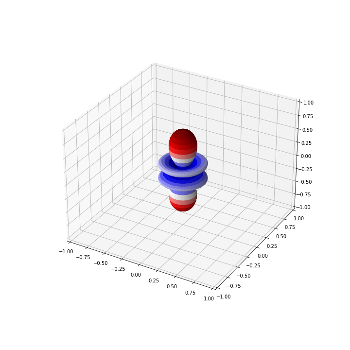
l = 3
m = 0
Ylm_num = 1/2 * abs(Ylm(l, m, theta, phi) + Ylm(l, -m, theta, phi)) 

Now, however, we still have a small problem because we want to represent our data points in a Cartesian coordinate system, but our grid points are defined in spherical coordinates. Therefore it is necessary to transform the calculated values of Ylm into the Cartesian coordinate system. The transformation reads:

x = np.cos(phi) * np.sin(theta) * Ylm_num
y = np.sin(phi) * np.sin(theta) * Ylm_num
z = np.cos(theta) * Ylm_num 

Now we have everything we need to represent the spherical harmonics in 3 dimensions. We do a little trick and map the data points to a number range from 0 to 1 and store these values in the variable colors. This allows us to colorize the spherical harmonics with a colormap from Matplotlib.

colors = Ylm_num / (Ylm_num.max() - Ylm_num.min())

fig = plt.figure(figsize=(10, 10))
ax = fig.add_subplot(111, projection="3d")

ax.plot_surface(x, y, z, facecolors=cm.seismic(colors))

ax.set_xlim([-1, 1])
ax.set_ylim([-1, 1])
ax.set_zlim([-1, 1])
fig.show() 

For the above example with \( Y_{30}\), the graph should look like